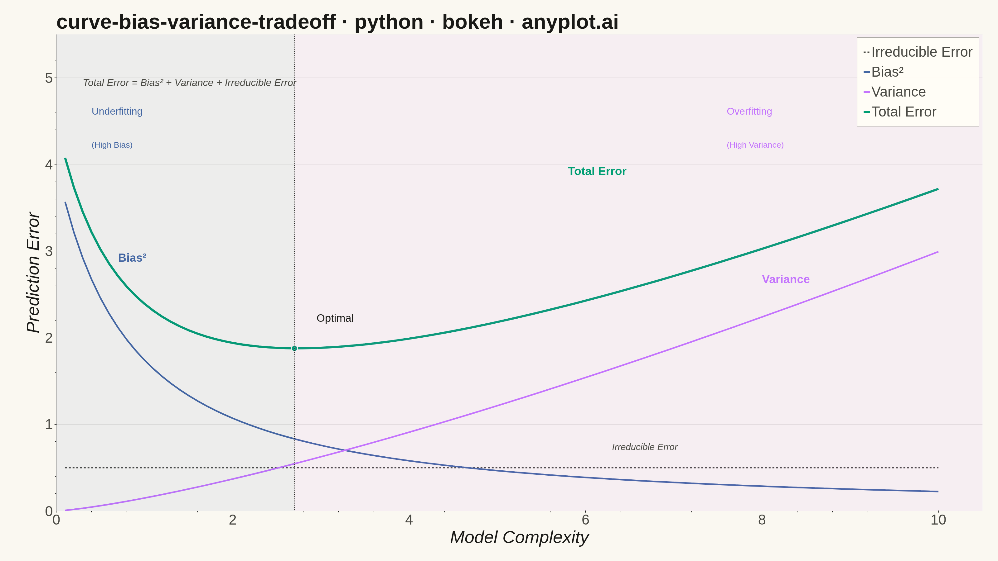
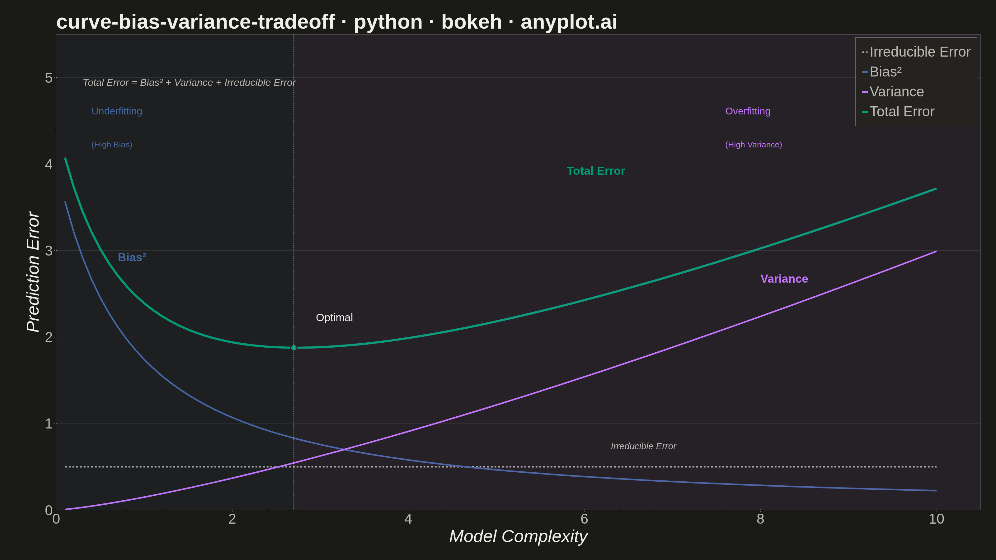
A theoretical visualization of the bias-variance tradeoff showing how total prediction error decomposes into bias squared, variance, and irreducible noise as a function of model complexity. The plot displays multiple curves: bias squared (decreasing with complexity), variance (increasing with complexity), irreducible error (constant), and total error (U-shaped). This is one of the most fundamental conceptual plots in machine learning for understanding model selection, overfitting, and underfitting.
""" anyplot.ai
curve-bias-variance-tradeoff: Bias-Variance Tradeoff Curve
Library: bokeh 3.9.0 | Python 3.13.13
Quality: 89/100 | Updated: 2026-05-28
"""

import os
import sys
import time
from pathlib import Path


# Remove the script's own directory from sys.path so 'bokeh' resolves to the
# installed package, not this file (bokeh.py in the same directory).
sys.path = [p for p in sys.path if os.path.abspath(p) != os.path.abspath(os.path.dirname(__file__) or ".")]

import numpy as np
from bokeh.io import output_file, save
from bokeh.models import BoxAnnotation, ColumnDataSource, Label, Span
from bokeh.plotting import figure
from selenium import webdriver
from selenium.webdriver.chrome.options import Options


# Theme tokens
THEME = os.getenv("ANYPLOT_THEME", "light")
PAGE_BG = "#FAF8F1" if THEME == "light" else "#1A1A17"
ELEVATED_BG = "#FFFDF6" if THEME == "light" else "#242420"
INK = "#1A1A17" if THEME == "light" else "#F0EFE8"
INK_SOFT = "#4A4A44" if THEME == "light" else "#B8B7B0"

# Imprint palette — semantic assignments for this spec
COLOR_TOTAL = "#009E73"  # brand green — first/most prominent (U-shaped key curve)
COLOR_BIAS = "#4467A3"  # blue — semantic fit with underfitting zone
COLOR_VARIANCE = "#C475FD"  # purple — second categorical

# Data — theoretical bias-variance tradeoff curves
np.random.seed(42)
complexity = np.linspace(0.1, 10, 100)

bias_squared = 4.0 / (1 + complexity) ** 1.2
variance = 0.15 * complexity**1.3
irreducible_error = np.full_like(complexity, 0.5)
total_error = bias_squared + variance + irreducible_error

optimal_idx = np.argmin(total_error)
optimal_complexity = complexity[optimal_idx]
optimal_error = total_error[optimal_idx]

source = ColumnDataSource(
    data={
        "complexity": complexity,
        "bias_squared": bias_squared,
        "variance": variance,
        "irreducible_error": irreducible_error,
        "total_error": total_error,
    }
)

# Plot
title_str = "curve-bias-variance-tradeoff · python · bokeh · anyplot.ai"

p = figure(
    width=3200,
    height=1800,
    title=title_str,
    x_axis_label="Model Complexity",
    y_axis_label="Prediction Error",
    x_range=(0, 10.5),
    y_range=(0, 5.5),
    toolbar_location=None,
    min_border_bottom=160,
    min_border_left=180,
    min_border_top=110,
    min_border_right=50,
)

# Shaded underfitting / overfitting zones
underfitting_zone = BoxAnnotation(left=0, right=optimal_complexity, fill_alpha=0.07, fill_color=COLOR_BIAS)
overfitting_zone = BoxAnnotation(left=optimal_complexity, right=11, fill_alpha=0.07, fill_color=COLOR_VARIANCE)
p.add_layout(underfitting_zone)
p.add_layout(overfitting_zone)

# Curves — drawn in order: background lines first, Total Error on top
p.line(
    "complexity",
    "irreducible_error",
    source=source,
    line_width=4,
    line_color=INK_SOFT,
    line_dash="dashed",
    legend_label="Irreducible Error",
)
p.line("complexity", "bias_squared", source=source, line_width=5, line_color=COLOR_BIAS, legend_label="Bias²")
p.line("complexity", "variance", source=source, line_width=5, line_color=COLOR_VARIANCE, legend_label="Variance")
p.line("complexity", "total_error", source=source, line_width=7, line_color=COLOR_TOTAL, legend_label="Total Error")

# Optimal complexity — vertical dotted guide + marker
optimal_line = Span(location=optimal_complexity, dimension="height", line_color=INK, line_width=2, line_dash="dotted")
p.add_layout(optimal_line)
p.scatter([optimal_complexity], [optimal_error], size=20, color=COLOR_TOTAL, line_color=PAGE_BG, line_width=3)

# Direct curve labels
p.add_layout(Label(x=0.7, y=2.85, text="Bias²", text_font_size="28pt", text_color=COLOR_BIAS, text_font_style="bold"))
p.add_layout(
    Label(x=8.0, y=2.6, text="Variance", text_font_size="28pt", text_color=COLOR_VARIANCE, text_font_style="bold")
)
p.add_layout(
    Label(x=6.3, y=0.68, text="Irreducible Error", text_font_size="22pt", text_color=INK_SOFT, text_font_style="italic")
)
p.add_layout(
    Label(x=5.8, y=3.85, text="Total Error", text_font_size="28pt", text_color=COLOR_TOTAL, text_font_style="bold")
)
p.add_layout(
    Label(x=optimal_complexity + 0.25, y=optimal_error + 0.28, text="Optimal", text_font_size="26pt", text_color=INK)
)

# Formula annotation
p.add_layout(
    Label(
        x=0.3,
        y=4.88,
        text="Total Error = Bias² + Variance + Irreducible Error",
        text_font_size="24pt",
        text_color=INK_SOFT,
        text_font_style="italic",
    )
)

# Zone labels (top corners of each region)
p.add_layout(Label(x=0.4, y=4.55, text="Underfitting", text_font_size="24pt", text_color=COLOR_BIAS))
p.add_layout(Label(x=0.4, y=4.17, text="(High Bias)", text_font_size="20pt", text_color=COLOR_BIAS))
p.add_layout(Label(x=7.6, y=4.55, text="Overfitting", text_font_size="24pt", text_color=COLOR_VARIANCE))
p.add_layout(Label(x=7.6, y=4.17, text="(High Variance)", text_font_size="20pt", text_color=COLOR_VARIANCE))

# Text sizing
p.title.text_font_size = "50pt"
p.title.text_font_style = "bold"
p.title.text_color = INK
p.xaxis.axis_label_text_font_size = "42pt"
p.yaxis.axis_label_text_font_size = "42pt"
p.xaxis.major_label_text_font_size = "34pt"
p.yaxis.major_label_text_font_size = "34pt"
p.xaxis.axis_label_text_color = INK
p.yaxis.axis_label_text_color = INK
p.xaxis.major_label_text_color = INK_SOFT
p.yaxis.major_label_text_color = INK_SOFT
p.xaxis.axis_line_color = INK_SOFT
p.yaxis.axis_line_color = INK_SOFT
p.xaxis.major_tick_line_color = INK_SOFT
p.yaxis.major_tick_line_color = INK_SOFT

# Grid — Y-axis grid only for line charts
p.xgrid.grid_line_color = None
p.ygrid.grid_line_color = INK
p.ygrid.grid_line_alpha = 0.12

# Background and chrome
p.background_fill_color = PAGE_BG
p.border_fill_color = PAGE_BG
p.outline_line_color = None

# Legend
p.legend.location = "top_right"
p.legend.label_text_font_size = "34pt"
p.legend.label_text_color = INK_SOFT
p.legend.background_fill_color = ELEVATED_BG
p.legend.border_line_color = INK_SOFT
p.legend.spacing = 12
p.legend.padding = 20

# Save HTML (interactive artifact) + PNG via headless Chrome
output_file(f"plot-{THEME}.html")
save(p)

# Window height is set ~140px taller than the figure so the viewport
# content area (figure height = 1800) isn't clipped by browser chrome.
W, H = 3200, 1940
opts = Options()
for arg in (
    "--headless=new",
    "--no-sandbox",
    "--disable-dev-shm-usage",
    "--disable-gpu",
    f"--window-size={W},{H}",
    "--hide-scrollbars",
):
    opts.add_argument(arg)
driver = webdriver.Chrome(options=opts)
driver.set_window_size(W, H)
driver.get(f"file://{Path(f'plot-{THEME}.html').resolve()}")
time.sleep(3)
driver.save_screenshot(f"plot-{THEME}.png")
driver.quit()
Runnable source as JSON, for any HTTP client: https://api.anyplot.ai/specs/curve-bias-variance-tradeoff/bokeh/code. Any spec id and library id listed in llms-full.txt fit the same URL shape; every URL below is complete and callable.
{
  "spec_id": "curve-bias-variance-tradeoff",
  "language": "python",
  "library": "bokeh",
  "page": "https://anyplot.ai/curve-bias-variance-tradeoff/python/bokeh",
  "hub": "https://anyplot.ai/curve-bias-variance-tradeoff",
  "code_json": "https://api.anyplot.ai/specs/curve-bias-variance-tradeoff/bokeh/code",
  "spec_json": "https://api.anyplot.ai/specs/curve-bias-variance-tradeoff",
  "render_light_png": "https://storage.googleapis.com/anyplot-images/plots/curve-bias-variance-tradeoff/python/bokeh/plot-light.png",
  "render_dark_png": "https://storage.googleapis.com/anyplot-images/plots/curve-bias-variance-tradeoff/python/bokeh/plot-dark.png",
  "interactive_light_html": "https://storage.googleapis.com/anyplot-images/plots/curve-bias-variance-tradeoff/python/bokeh/plot-light.html",
  "interactive_dark_html": "https://storage.googleapis.com/anyplot-images/plots/curve-bias-variance-tradeoff/python/bokeh/plot-dark.html",
  "quality_score": 89.0,
  "license": "MIT",
  "guide": "https://anyplot.ai/llms.txt"
}
Part of Bias-Variance Tradeoff Curve on anyplot.ai.