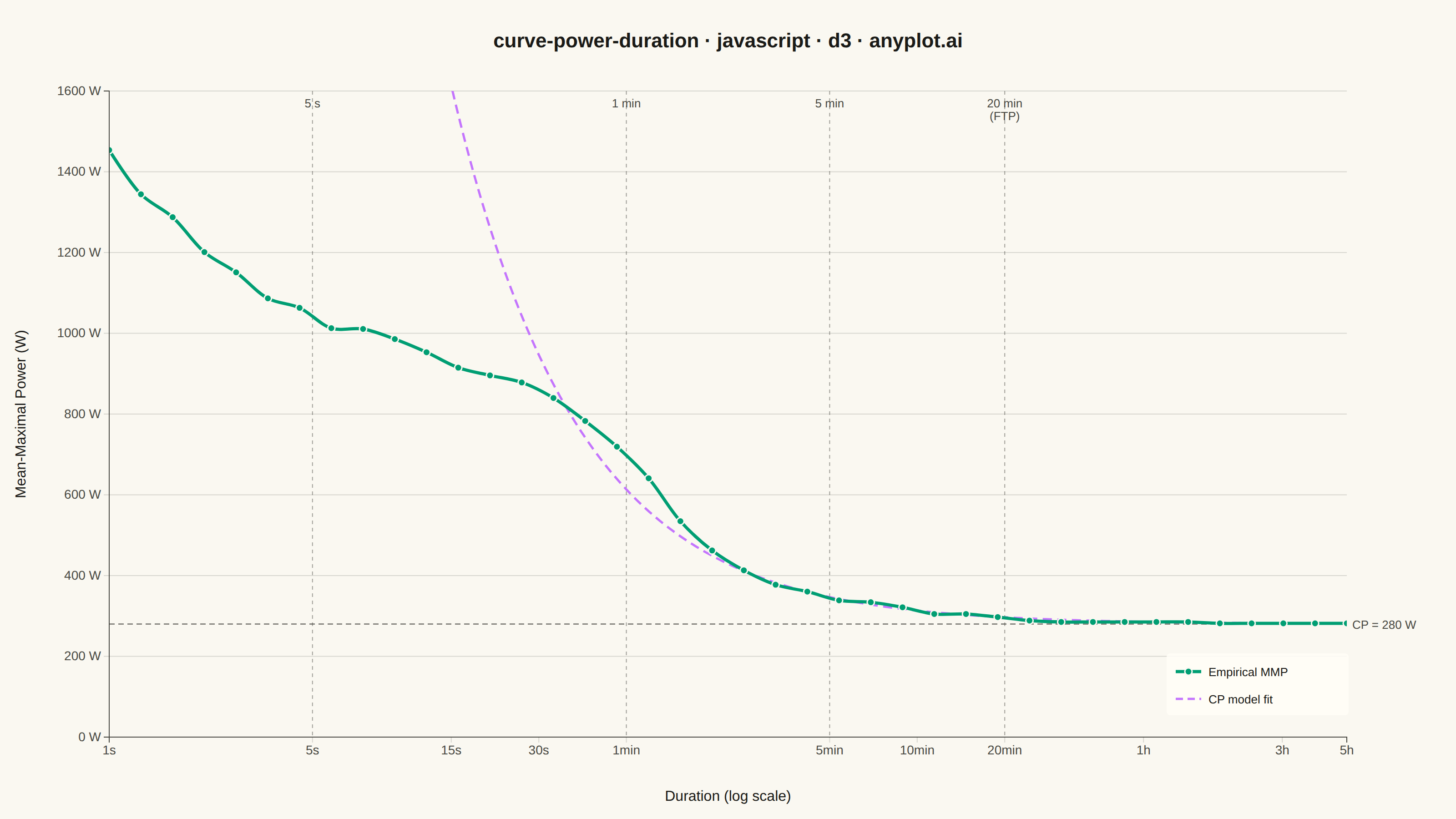
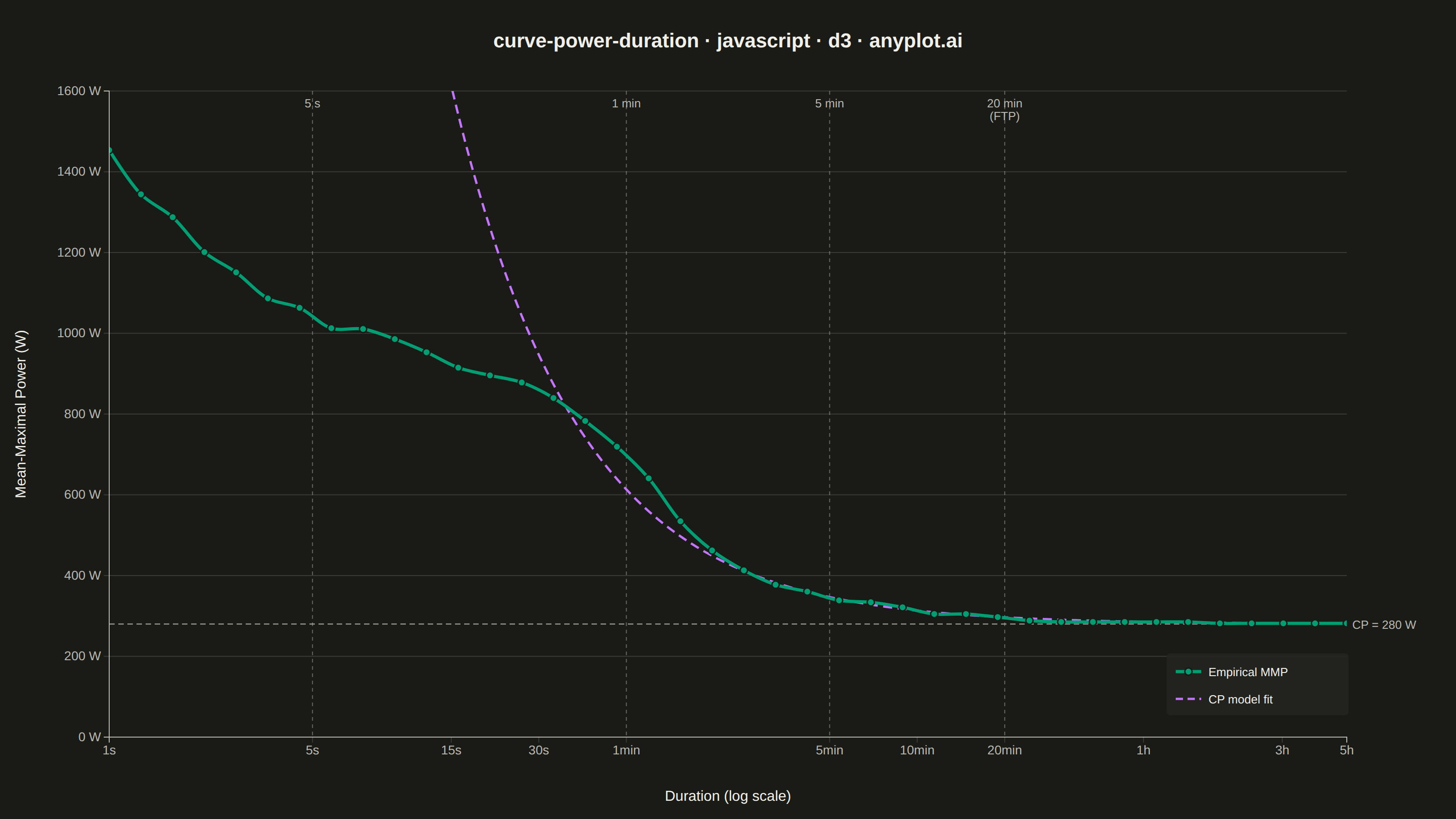
A power duration curve plots an athlete's best mean-maximal power output (watts) against effort duration on a logarithmic time axis spanning roughly 1 second to several hours. Each point answers "what is the highest average power this rider could sustain for exactly this long?", producing a characteristic monotonically decreasing decay curve. A critical power (CP) model is fitted and overlaid, decomposing performance into an aerobic asymptote (CP) and a finite anaerobic work capacity (W′). The chart is a cornerstone of cycling and endurance sports analytics for profiling rider strengths, tracking fitness, and setting training zones.
// anyplot.ai
// curve-power-duration: Mean-Maximal Power Duration Curve
// Library: d3 7.9.0 | JavaScript 22.22.3
// Quality: 90/100 | Created: 2026-06-13

const t = window.ANYPLOT_TOKENS;
const { width, height } = window.ANYPLOT_SIZE;
const margin = { top: 100, right: 120, bottom: 90, left: 120 };
const iw = width - margin.left - margin.right;
const ih = height - margin.top - margin.bottom;

// --- Data: synthetic well-trained cyclist, CP = 280 W, W' = 20 000 J ---
// Empirical MMP peaks near 1100 W at 1 s (neuromuscular ceiling); the simple
// CP model P = CP + W'/t diverges to ~20 000 W at 1 s and is shown clipped.
const CP = 280;
const Wp = 20000;

function logspace(a, b, n) {
  const la = Math.log10(a), lb = Math.log10(b);
  return Array.from({ length: n }, (_, i) => Math.pow(10, la + (lb - la) * i / (n - 1)));
}

const durations = logspace(1, 18000, 40);

// Deterministic LCG for reproducible noise
let lcgState = 42;
function lcg() {
  lcgState = (lcgState * 1664525 + 1013904223) & 0xffffffff;
  return (lcgState >>> 0) / 4294967295;
}

// Physiological empirical model: neuro-muscular ceiling fading into CP model
// - Short efforts (<~60 s): dominated by neuro peak (~1100 W at 1 s)
// - Long efforts (>~120 s): converges to CP + W'/t
function empiricalBase(dur) {
  const cpModel = CP + Wp / dur;
  const neuro = 1100 * Math.pow(dur, -0.08);   // power-law decay from neuromuscular peak
  const blend = 1 / (1 + Math.exp((dur - 60) / 15));  // sigmoid: 1 at short, 0 at long
  return neuro * blend + cpModel * (1 - blend);
}

const rawPower = durations.map(dur => empiricalBase(dur) * (1 + (lcg() - 0.5) * 0.04));
const empiricalPower = rawPower.slice();
for (let i = 1; i < empiricalPower.length; i++) {
  empiricalPower[i] = Math.min(empiricalPower[i], empiricalPower[i - 1]);
}

// Smooth CP model line (more points)
const modelDurs = logspace(1, 18000, 300);
const modelPow = modelDurs.map(dur => CP + Wp / dur);

// --- SVG setup ---
const svg = d3.select("#container")
  .append("svg")
  .attr("width", width)
  .attr("height", height);

const g = svg.append("g")
  .attr("transform", `translate(${margin.left},${margin.top})`);

// --- Scales ---
const xScale = d3.scaleLog().domain([1, 18000]).range([0, iw]);
const yMax = Math.ceil(d3.max(empiricalPower) / 100) * 100 + 100;
const yScale = d3.scaleLinear().domain([0, yMax]).range([ih, 0]);

// --- Clip path so the diverging model line stays inside the plot area ---
svg.append("defs").append("clipPath").attr("id", "plot-clip")
  .append("rect").attr("width", iw).attr("height", ih);

// --- Y-axis grid ---
g.selectAll(".grid-y").data(yScale.ticks(6)).join("line")
  .attr("x1", 0).attr("x2", iw)
  .attr("y1", d => yScale(d)).attr("y2", d => yScale(d))
  .attr("stroke", t.grid).attr("stroke-width", 1);

// --- Reference duration markers ---
const refs = [
  { dur: 5, line1: "5 s", line2: null },
  { dur: 60, line1: "1 min", line2: null },
  { dur: 300, line1: "5 min", line2: null },
  { dur: 1200, line1: "20 min", line2: "(FTP)" },
];

refs.forEach(ref => {
  const rx = xScale(ref.dur);
  g.append("line")
    .attr("x1", rx).attr("x2", rx)
    .attr("y1", 0).attr("y2", ih)
    .attr("stroke", t.inkSoft)
    .attr("stroke-width", 1)
    .attr("stroke-dasharray", "4,4")
    .attr("opacity", 0.5);
  g.append("text")
    .attr("x", rx).attr("y", 18)
    .attr("text-anchor", "middle")
    .attr("fill", t.inkSoft)
    .style("font-size", "13px")
    .text(ref.line1);
  if (ref.line2) {
    g.append("text")
      .attr("x", rx).attr("y", 32)
      .attr("text-anchor", "middle")
      .attr("fill", t.inkSoft)
      .style("font-size", "13px")
      .text(ref.line2);
  }
});

// --- CP horizontal asymptote ---
g.append("line")
  .attr("x1", 0).attr("x2", iw)
  .attr("y1", yScale(CP)).attr("y2", yScale(CP))
  .attr("stroke", t.inkSoft)
  .attr("stroke-width", 1.5)
  .attr("stroke-dasharray", "6,4")
  .attr("opacity", 0.65);
g.append("text")
  .attr("x", iw + 6).attr("y", yScale(CP) + 5)
  .attr("fill", t.inkSoft)
  .style("font-size", "13px")
  .text(`CP = ${CP} W`);

// --- Model fit line (dashed, Imprint palette[1]) — clipped to plot area ---
const modelLine = d3.line()
  .x(d => xScale(d.dur))
  .y(d => yScale(d.pow))
  .curve(d3.curveCatmullRom.alpha(0.5));

g.append("path")
  .datum(modelDurs.map((dur, i) => ({ dur, pow: modelPow[i] })))
  .attr("clip-path", "url(#plot-clip)")
  .attr("fill", "none")
  .attr("stroke", t.palette[1])
  .attr("stroke-width", 2.5)
  .attr("stroke-dasharray", "10,6")
  .attr("d", modelLine);

// --- Empirical MMP curve (solid, Imprint palette[0] — always first series) ---
const empirLine = d3.line()
  .x((d, i) => xScale(durations[i]))
  .y(d => yScale(d))
  .curve(d3.curveCatmullRom.alpha(0.5));

g.append("path")
  .datum(empiricalPower)
  .attr("clip-path", "url(#plot-clip)")
  .attr("fill", "none")
  .attr("stroke", t.palette[0])
  .attr("stroke-width", 3.5)
  .attr("d", empirLine);

// Dots on empirical curve
g.selectAll(".dot").data(empiricalPower).join("circle")
  .attr("clip-path", "url(#plot-clip)")
  .attr("cx", (d, i) => xScale(durations[i]))
  .attr("cy", d => yScale(d))
  .attr("r", 4)
  .attr("fill", t.palette[0])
  .attr("stroke", t.pageBg)
  .attr("stroke-width", 1.5);

// --- X-axis (log scale, human-readable tick labels) ---
const xTickVals = [1, 5, 15, 30, 60, 300, 600, 1200, 3600, 10800, 18000];
const xTickFmt = s => {
  if (s < 60) return `${s}s`;
  if (s < 3600) return `${s / 60}min`;
  return `${s / 3600}h`;
};

const xAxis = g.append("g")
  .attr("transform", `translate(0,${ih})`)
  .call(d3.axisBottom(xScale).tickValues(xTickVals).tickFormat(xTickFmt));
xAxis.selectAll("text").attr("fill", t.inkSoft).style("font-size", "14px");
xAxis.selectAll("line").attr("stroke", t.grid);
xAxis.select(".domain").attr("stroke", t.inkSoft);

// --- Y-axis ---
const yAxis = g.append("g")
  .call(d3.axisLeft(yScale).ticks(6).tickFormat(d => `${Math.round(d)} W`));
yAxis.selectAll("text").attr("fill", t.inkSoft).style("font-size", "14px");
yAxis.selectAll("line").attr("stroke", t.grid);
yAxis.select(".domain").attr("stroke", t.inkSoft);

// --- Axis labels ---
svg.append("text")
  .attr("x", margin.left + iw / 2)
  .attr("y", height - 20)
  .attr("text-anchor", "middle")
  .attr("fill", t.ink)
  .style("font-size", "16px")
  .text("Duration (log scale)");

svg.append("text")
  .attr("transform", `translate(28, ${margin.top + ih / 2}) rotate(-90)`)
  .attr("text-anchor", "middle")
  .attr("fill", t.ink)
  .style("font-size", "16px")
  .text("Mean-Maximal Power (W)");

// --- Legend ---
const legX = iw - 188;
const legY = ih - 82;

g.append("rect")
  .attr("x", legX - 10).attr("y", legY - 10)
  .attr("width", 200).attr("height", 68)
  .attr("fill", t.elevatedBg).attr("rx", 4)
  .attr("opacity", 0.9);

g.append("line")
  .attr("x1", legX).attr("x2", legX + 28)
  .attr("y1", legY + 10).attr("y2", legY + 10)
  .attr("stroke", t.palette[0]).attr("stroke-width", 3.5);
g.append("circle")
  .attr("cx", legX + 14).attr("cy", legY + 10).attr("r", 4)
  .attr("fill", t.palette[0]).attr("stroke", t.pageBg).attr("stroke-width", 1.5);
g.append("text")
  .attr("x", legX + 36).attr("y", legY + 15)
  .attr("fill", t.ink).style("font-size", "13px")
  .text("Empirical MMP");

g.append("line")
  .attr("x1", legX).attr("x2", legX + 28)
  .attr("y1", legY + 40).attr("y2", legY + 40)
  .attr("stroke", t.palette[1]).attr("stroke-width", 2.5)
  .attr("stroke-dasharray", "8,5");
g.append("text")
  .attr("x", legX + 36).attr("y", legY + 45)
  .attr("fill", t.ink).style("font-size", "13px")
  .text("CP model fit");

// --- Title ---
svg.append("text")
  .attr("x", width / 2).attr("y", 52)
  .attr("text-anchor", "middle")
  .attr("fill", t.ink)
  .style("font-size", "22px")
  .style("font-weight", "600")
  .text("curve-power-duration · javascript · d3 · anyplot.ai");
Runnable source as JSON, for any HTTP client: https://api.anyplot.ai/specs/curve-power-duration/d3/code. Any spec id and library id listed in llms-full.txt fit the same URL shape; every URL below is complete and callable.
{
  "spec_id": "curve-power-duration",
  "language": "javascript",
  "library": "d3",
  "page": "https://anyplot.ai/curve-power-duration/javascript/d3",
  "hub": "https://anyplot.ai/curve-power-duration",
  "code_json": "https://api.anyplot.ai/specs/curve-power-duration/d3/code",
  "spec_json": "https://api.anyplot.ai/specs/curve-power-duration",
  "render_light_png": "https://storage.googleapis.com/anyplot-images/plots/curve-power-duration/javascript/d3/plot-light.png",
  "render_dark_png": "https://storage.googleapis.com/anyplot-images/plots/curve-power-duration/javascript/d3/plot-dark.png",
  "interactive_light_html": "https://storage.googleapis.com/anyplot-images/plots/curve-power-duration/javascript/d3/plot-light.html",
  "interactive_dark_html": "https://storage.googleapis.com/anyplot-images/plots/curve-power-duration/javascript/d3/plot-dark.html",
  "quality_score": 90.0,
  "license": "MIT",
  "guide": "https://anyplot.ai/llms.txt"
}
Part of Mean-Maximal Power Duration Curve on anyplot.ai.