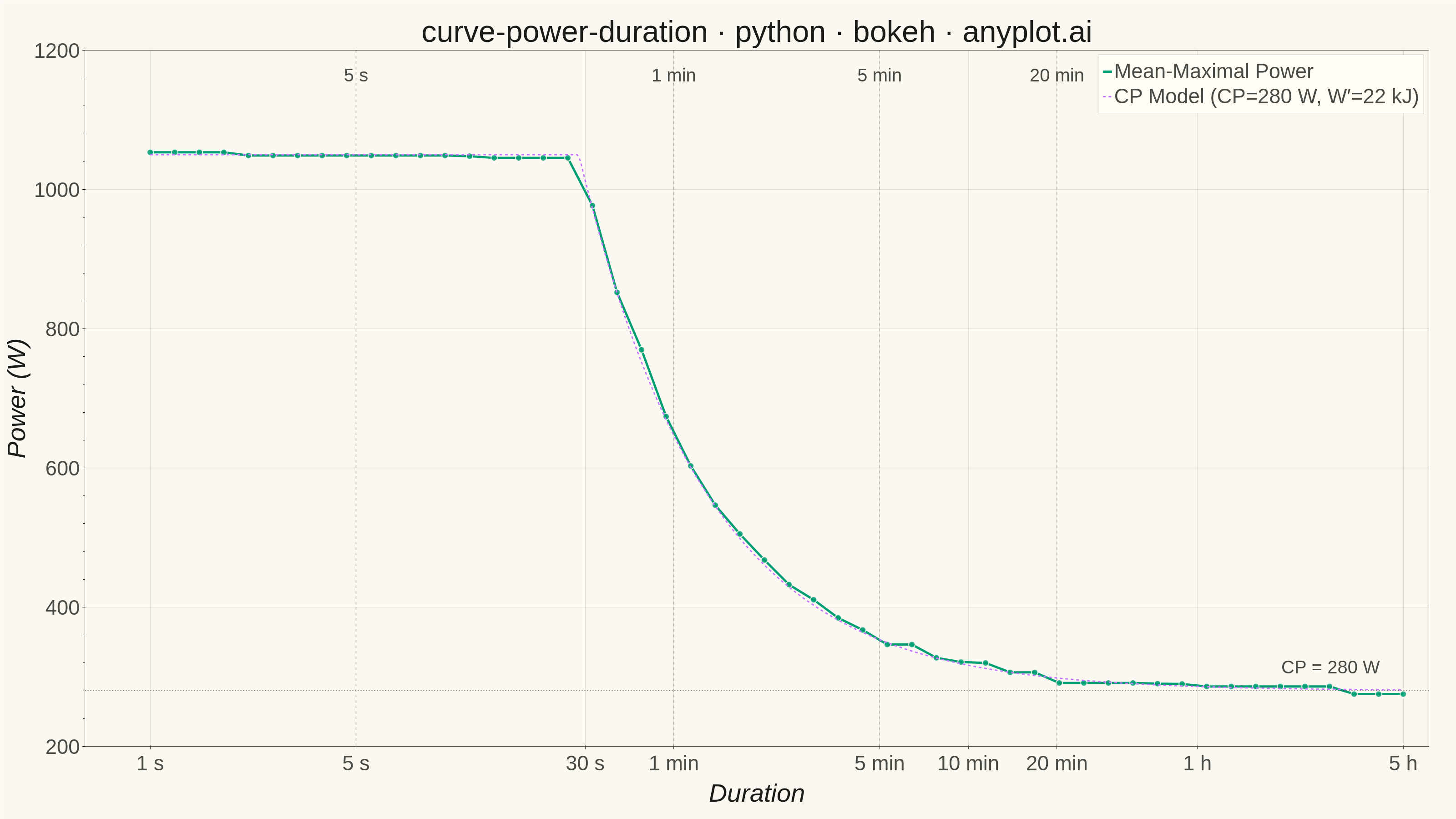
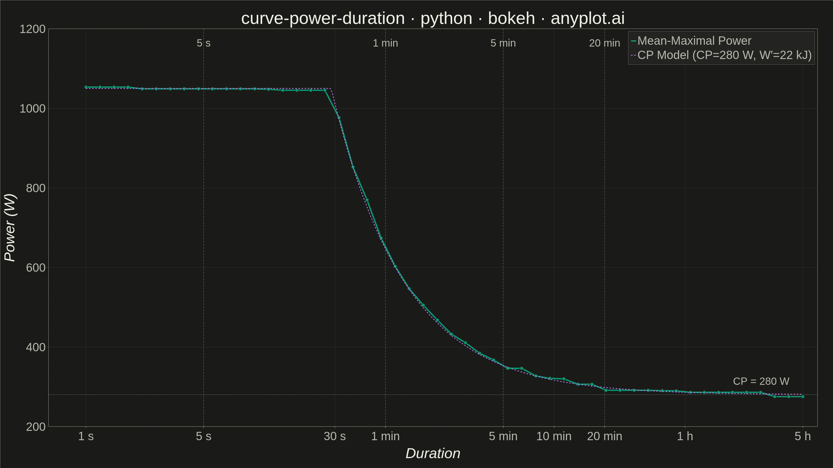
A power duration curve plots an athlete's best mean-maximal power output (watts) against effort duration on a logarithmic time axis spanning roughly 1 second to several hours. Each point answers "what is the highest average power this rider could sustain for exactly this long?", producing a characteristic monotonically decreasing decay curve. A critical power (CP) model is fitted and overlaid, decomposing performance into an aerobic asymptote (CP) and a finite anaerobic work capacity (W′). The chart is a cornerstone of cycling and endurance sports analytics for profiling rider strengths, tracking fitness, and setting training zones.
""" anyplot.ai
curve-power-duration: Mean-Maximal Power Duration Curve
Library: bokeh 3.9.1 | Python 3.13.13
Quality: 89/100 | Created: 2026-06-13
"""

import os
import time
from pathlib import Path

import numpy as np
from bokeh.io import output_file, save
from bokeh.models import ColumnDataSource, CustomJSTickFormatter, FixedTicker, Label, Range1d, Span
from bokeh.plotting import figure
from selenium import webdriver
from selenium.webdriver.chrome.options import Options


# Theme tokens
THEME = os.getenv("ANYPLOT_THEME", "light")
PAGE_BG = "#FAF8F1" if THEME == "light" else "#1A1A17"
ELEVATED_BG = "#FFFDF6" if THEME == "light" else "#242420"
INK = "#1A1A17" if THEME == "light" else "#F0EFE8"
INK_SOFT = "#4A4A44" if THEME == "light" else "#B8B7B0"
INK_MUTED = "#6B6A63" if THEME == "light" else "#A8A79F"

# Imprint palette — canonical order; positions 1 and 2 for the two data series
BRAND = "#009E73"  # position 1 — empirical mean-maximal curve (always first)
MODEL_COLOR = "#C475FD"  # position 2 — fitted CP model line

# Data — well-trained competitive cyclist
np.random.seed(42)
CP_VAL = 280  # Critical Power in watts (aerobic ceiling)
WPRIME = 22000  # W' anaerobic work capacity in joules
PMAX = 1050  # Neuromuscular peak power (sprint ceiling, ~1 s effort)

# Log-spaced effort durations: 1 s → 18,000 s (5 h)
durations = np.logspace(0, np.log10(18000), 52)

# CP model: P(t) = CP + W'/t, capped at neuromuscular maximum
model_power = np.minimum(PMAX, CP_VAL + WPRIME / durations)

# Empirical mean-maximal power: slight positive scatter around model
noise = np.random.normal(0, 5, len(durations))
empirical_power = model_power + noise + np.random.uniform(0, 12, len(durations))
empirical_power = np.clip(empirical_power, model_power * 0.97, model_power * 1.03)
# Enforce monotonically non-increasing (best average power always drops with duration)
for i in range(1, len(empirical_power)):
    empirical_power[i] = min(empirical_power[i], empirical_power[i - 1])

# Dense smooth curve for the model overlay
durations_dense = np.logspace(0, np.log10(18000), 400)
model_dense = np.minimum(PMAX, CP_VAL + WPRIME / durations_dense)

# Reference annotation durations (per specification)
ref_durations = {"5 s": 5, "1 min": 60, "5 min": 300, "20 min": 1200}

# Title (50 chars — within 67-char baseline; default font size applies)
title = "curve-power-duration · python · bokeh · anyplot.ai"

# Figure — landscape 3200×1800, log x-axis
p = figure(
    width=3200,
    height=1800,
    title=title,
    x_axis_label="Duration",
    y_axis_label="Power (W)",
    x_axis_type="log",
    x_range=(0.6, 22000),
    y_range=Range1d(200, 1200),
    toolbar_location=None,
    min_border_bottom=160,
    min_border_left=180,
    min_border_top=110,
    min_border_right=60,
)

# Empirical mean-maximal power (primary series — BRAND green, always first)
src_emp = ColumnDataSource({"x": durations, "y": empirical_power})
p.line("x", "y", source=src_emp, line_color=BRAND, line_width=5, line_alpha=0.7, legend_label="Mean-Maximal Power")
p.scatter("x", "y", source=src_emp, color=BRAND, size=14, alpha=0.85, line_color=PAGE_BG, line_width=2)

# Fitted CP model overlay — dashed, secondary series color
src_mdl = ColumnDataSource({"x": durations_dense, "y": model_dense})
p.line(
    "x",
    "y",
    source=src_mdl,
    line_color=MODEL_COLOR,
    line_width=5,
    line_dash="dashed",
    legend_label=f"CP Model (CP={CP_VAL} W, W′=22 kJ)",
)

# CP asymptote — neutral dotted horizontal reference line
p.add_layout(
    Span(location=CP_VAL, dimension="width", line_color=INK_SOFT, line_width=2, line_dash="dotted", line_alpha=0.75)
)

# Vertical reference markers at key durations
for t in ref_durations.values():
    p.add_layout(
        Span(location=t, dimension="height", line_color=INK_MUTED, line_width=1.5, line_dash="dashed", line_alpha=0.5)
    )

# Reference duration labels near the top of the plot
for label, t in ref_durations.items():
    p.add_layout(
        Label(
            x=t,
            y=1150,
            text=label,
            text_font_size="34pt",
            text_color=INK_SOFT,
            text_align="center",
            text_baseline="bottom",
            x_units="data",
            y_units="data",
        )
    )

# CP asymptote label (right side)
p.add_layout(
    Label(
        x=15000,
        y=CP_VAL + 20,
        text=f"CP = {CP_VAL} W",
        text_font_size="34pt",
        text_color=INK_SOFT,
        text_align="right",
        text_baseline="bottom",
        x_units="data",
        y_units="data",
    )
)

# Log x-axis: human-readable tick labels
p.xaxis.ticker = FixedTicker(ticks=[1, 5, 30, 60, 300, 600, 1200, 3600, 18000])
p.xaxis.formatter = CustomJSTickFormatter(
    code="""
    var labels = {1: '1 s', 5: '5 s', 30: '30 s', 60: '1 min',
                  300: '5 min', 600: '10 min', 1200: '20 min',
                  3600: '1 h', 18000: '5 h'};
    return labels[tick] || String(tick);
    """
)

# Theme-adaptive chrome
p.background_fill_color = PAGE_BG
p.border_fill_color = PAGE_BG
p.outline_line_color = None

p.title.text_color = INK
p.title.text_font_size = "50pt"
p.title.text_font_style = "normal"
p.title.align = "center"

p.xaxis.axis_label_text_color = INK
p.yaxis.axis_label_text_color = INK
p.xaxis.axis_label_text_font_size = "42pt"
p.yaxis.axis_label_text_font_size = "42pt"

p.xaxis.major_label_text_color = INK_SOFT
p.yaxis.major_label_text_color = INK_SOFT
p.xaxis.major_label_text_font_size = "34pt"
p.yaxis.major_label_text_font_size = "34pt"

p.xaxis.axis_line_color = INK_SOFT
p.yaxis.axis_line_color = INK_SOFT
p.xaxis.major_tick_line_color = INK_SOFT
p.yaxis.major_tick_line_color = INK_SOFT

p.xgrid.grid_line_color = INK
p.ygrid.grid_line_color = INK
p.xgrid.grid_line_alpha = 0.12
p.ygrid.grid_line_alpha = 0.12

p.legend.background_fill_color = ELEVATED_BG
p.legend.border_line_color = INK_SOFT
p.legend.label_text_color = INK_SOFT
p.legend.label_text_font_size = "34pt"
p.legend.location = "top_right"

# Save interactive HTML artifact
output_file(f"plot-{THEME}.html")
save(p)

# Screenshot via headless Chrome (Selenium 4 / Selenium Manager)
W, H = 3200, 1800
opts = Options()
for arg in (
    "--headless=new",
    "--no-sandbox",
    "--disable-dev-shm-usage",
    "--disable-gpu",
    f"--window-size={W},{H}",
    "--hide-scrollbars",
):
    opts.add_argument(arg)
driver = webdriver.Chrome(options=opts)
# CDP override pins the viewport to exactly W×H at DPR=1, avoiding
# headless-Chrome viewport-vs-window-size discrepancies
driver.execute_cdp_cmd(
    "Emulation.setDeviceMetricsOverride", {"width": W, "height": H, "deviceScaleFactor": 1, "mobile": False}
)
driver.get(f"file://{Path(f'plot-{THEME}.html').resolve()}")
time.sleep(3)
driver.save_screenshot(f"plot-{THEME}.png")
driver.quit()
Runnable source as JSON, for any HTTP client: https://api.anyplot.ai/specs/curve-power-duration/bokeh/code. Any spec id and library id listed in llms-full.txt fit the same URL shape; every URL below is complete and callable.
{
  "spec_id": "curve-power-duration",
  "language": "python",
  "library": "bokeh",
  "page": "https://anyplot.ai/curve-power-duration/python/bokeh",
  "hub": "https://anyplot.ai/curve-power-duration",
  "code_json": "https://api.anyplot.ai/specs/curve-power-duration/bokeh/code",
  "spec_json": "https://api.anyplot.ai/specs/curve-power-duration",
  "render_light_png": "https://storage.googleapis.com/anyplot-images/plots/curve-power-duration/python/bokeh/plot-light.png",
  "render_dark_png": "https://storage.googleapis.com/anyplot-images/plots/curve-power-duration/python/bokeh/plot-dark.png",
  "interactive_light_html": "https://storage.googleapis.com/anyplot-images/plots/curve-power-duration/python/bokeh/plot-light.html",
  "interactive_dark_html": "https://storage.googleapis.com/anyplot-images/plots/curve-power-duration/python/bokeh/plot-dark.html",
  "quality_score": 89.0,
  "license": "MIT",
  "guide": "https://anyplot.ai/llms.txt"
}
Part of Mean-Maximal Power Duration Curve on anyplot.ai.