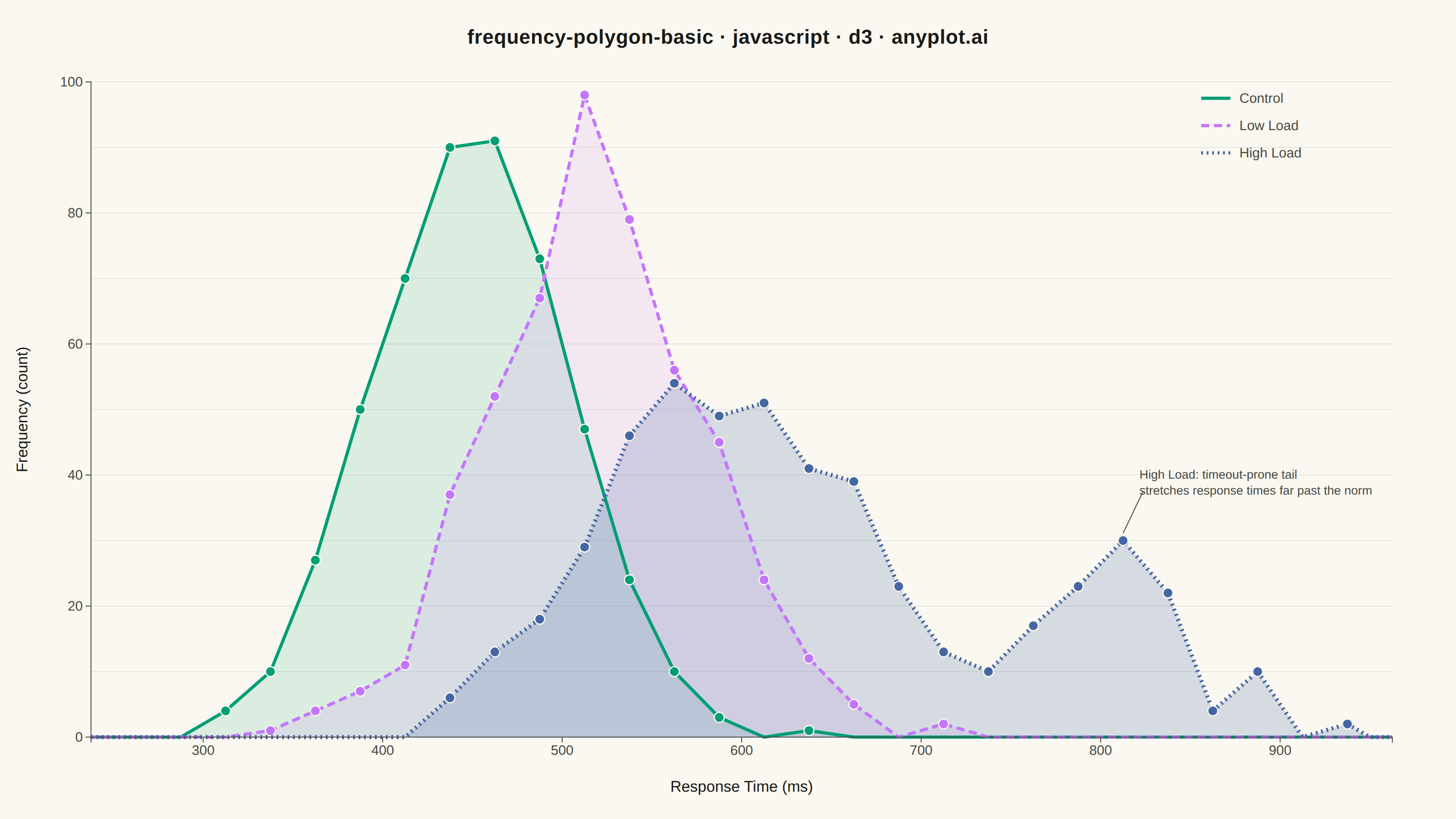
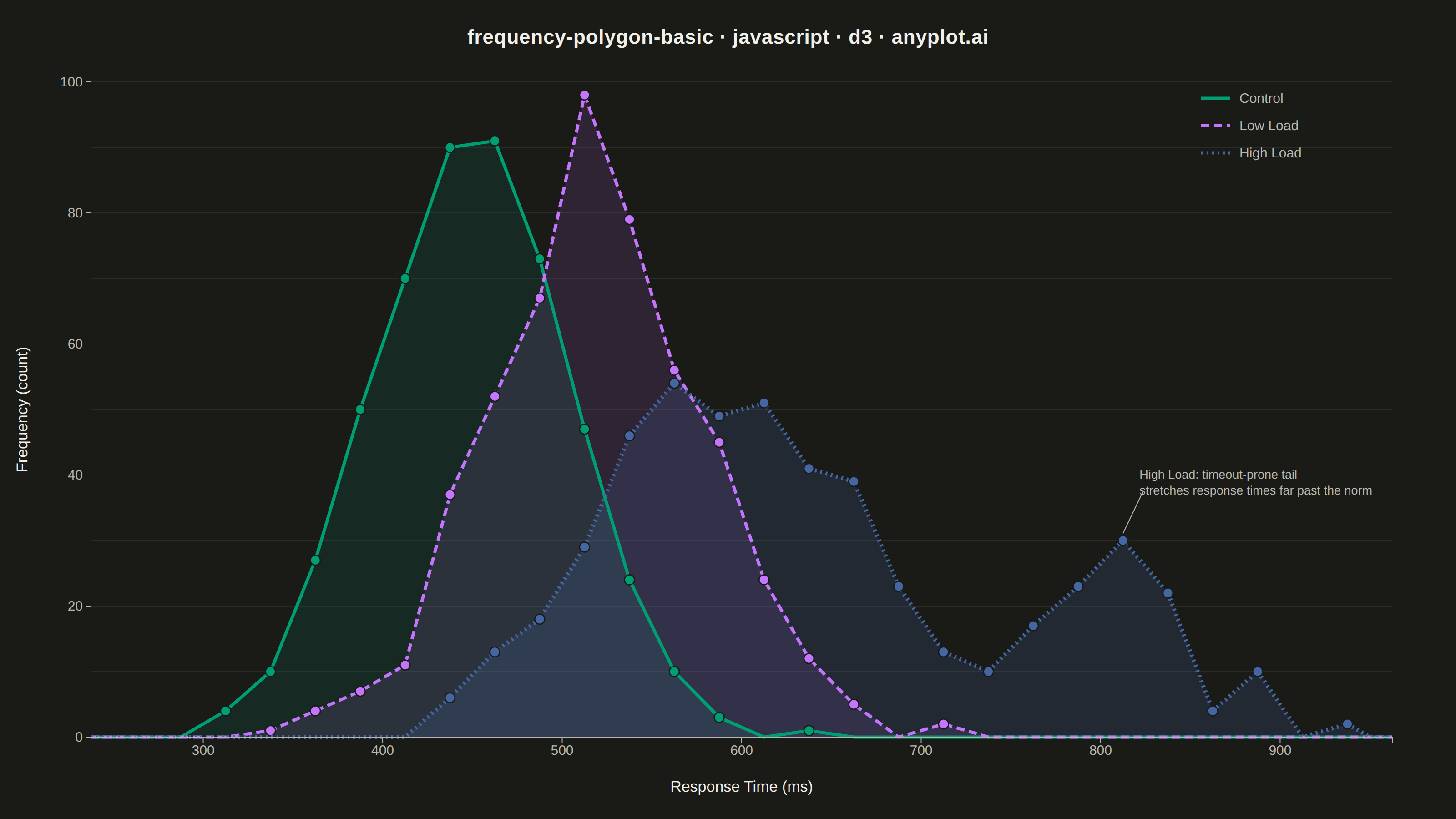
The same plot in 14 other libraries — JavaScript: Chart.js, Apache ECharts, Highcharts, MUI X Charts; Python: Altair, Bokeh, lets-plot, Matplotlib, Plotly, plotnine, Pygal, Seaborn; R: ggplot2; Julia: Makie.jl. Compare all 15 side by side: Frequency Polygon for Distribution Comparison in Python, R, Julia and JavaScript.
A frequency polygon connects the midpoints of histogram bins with straight line segments, creating an outline of the distribution shape. This visualization excels at comparing multiple distributions simultaneously since lines overlap without obscuring each other, unlike stacked or overlapping histogram bars. Frequency polygons reveal differences in central tendency, spread, skewness, and modality across groups with minimal visual clutter.
// anyplot.ai
// frequency-polygon-basic: Frequency Polygon for Distribution Comparison
// Library: d3 7.9.0 | JavaScript 22.23.2
// Quality: 91/100 | Created: 2026-09-02

const t = window.ANYPLOT_TOKENS;
const { width, height } = window.ANYPLOT_SIZE;
const margin = { top: 90, right: 70, bottom: 90, left: 100 };
const iw = width - margin.left - margin.right;
const ih = height - margin.top - margin.bottom;

// --- Data (in-memory, deterministic) ----------------------------------------
// Fixed-seed LCG — the browser has no seeded RNG.
const lcg = (seed) => {
  let state = seed >>> 0;
  return () => {
    state = (state * 1664525 + 1013904223) >>> 0;
    return state / 4294967296;
  };
};
const rng = lcg(42);
const randNormal = (mean, sd) => {
  const u1 = Math.max(rng(), 1e-9);
  const u2 = rng();
  const z = Math.sqrt(-2 * Math.log(u1)) * Math.cos(2 * Math.PI * u2);
  return mean + z * sd;
};

// High Load carries a secondary bump: under sustained load a fraction of
// requests hit retry/timeout queues, producing a long, right-skewed tail
// on top of the base slowdown — a shape difference plain mean/sd shift
// can't show, which is exactly what a frequency polygon is good at revealing.
const groups = [
  { name: "Control", mean: 450, sd: 55, n: 500, dash: "0" },
  { name: "Low Load", mean: 520, sd: 65, n: 500, dash: "9,5" },
  {
    name: "High Load",
    mean: 590,
    sd: 70,
    n: 500,
    dash: "2,4",
    bump: { mean: 800, sd: 45, weight: 0.22 },
    focal: true,
  },
];

const binMin = 250;
const binMax = 950;
const binWidth = 25;
const thresholds = d3.range(binMin, binMax + binWidth, binWidth);
const bin = d3.bin().domain([binMin, binMax]).thresholds(thresholds);

const sampleValue = (g) => (g.bump && rng() < g.bump.weight ? randNormal(g.bump.mean, g.bump.sd) : randNormal(g.mean, g.sd));

const series = groups.map((g, i) => {
  const values = Array.from({ length: g.n }, () => sampleValue(g)).filter(
    (v) => v > binMin && v < binMax,
  );
  const bins = bin(values);
  const midpoints = bins.map((b) => ({ x: (b.x0 + b.x1) / 2, y: b.length }));
  // Extend to zero at both ends to close the polygon shape.
  const points = [{ x: binMin - binWidth / 2, y: 0 }, ...midpoints, { x: binMax + binWidth / 2, y: 0 }];
  return { ...g, points, midpoints, color: t.palette[i] };
});

// --- Scales -------------------------------------------------------------------
const allPoints = series.flatMap((s) => s.points);
const x = d3
  .scaleLinear()
  .domain(d3.extent(allPoints, (d) => d.x))
  .range([0, iw]);
const y = d3
  .scaleLinear()
  .domain([0, d3.max(allPoints, (d) => d.y)])
  .nice()
  .range([ih, 0]);

// --- SVG mount ------------------------------------------------------------------
const svg = d3.select("#container").append("svg").attr("width", width).attr("height", height);
const g = svg.append("g").attr("transform", `translate(${margin.left},${margin.top})`);

// --- Y gridlines (subtle, behind data) -------------------------------------------
g.append("g")
  .call(d3.axisLeft(y).tickSize(-iw).tickFormat(""))
  .call((sel) => sel.select(".domain").remove())
  .selectAll("line")
  .attr("stroke", t.grid)
  .attr("stroke-opacity", 0.5);

// --- Area fills + polygon lines + markers ----------------------------------------
const area = d3
  .area()
  .x((d) => x(d.x))
  .y0(y(0))
  .y1((d) => y(d.y))
  .curve(d3.curveLinear);

const line = d3
  .line()
  .x((d) => x(d.x))
  .y((d) => y(d.y))
  .curve(d3.curveLinear);

for (const s of series) {
  g.append("path")
    .datum(s.points)
    .attr("d", area)
    .attr("fill", s.color)
    .attr("fill-opacity", s.focal ? 0.2 : 0.12);
}
for (const s of series) {
  g.append("path")
    .datum(s.points)
    .attr("d", line)
    .attr("fill", "none")
    .attr("stroke", s.color)
    .attr("stroke-width", s.focal ? 4.5 : 3.5)
    .attr("stroke-dasharray", s.dash)
    .attr("stroke-linejoin", "round");
  g.selectAll(`.marker-${s.name.replace(/\s+/g, "")}`)
    .data(s.midpoints.filter((d) => d.y > 0))
    .join("circle")
    .attr("cx", (d) => x(d.x))
    .attr("cy", (d) => y(d.y))
    .attr("r", 5.5)
    .attr("fill", s.color)
    .attr("stroke", t.pageBg)
    .attr("stroke-width", 1.3);
}

// --- Insight callout on the High Load tail bump (d3.greatest, d3-array) ------------
// A distinctive, non-generic use of d3 beyond bin/area/line: locate the
// secondary-bump peak precisely instead of hard-coding its screen position.
const highLoad = series.find((s) => s.name === "High Load");
const tailPeak = d3.greatest(
  highLoad.midpoints.filter((d) => d.x > 700 && d.y > 0),
  (d) => d.y,
);
if (tailPeak) {
  const px = x(tailPeak.x);
  const py = y(tailPeak.y);
  const lx = px + 18;
  const ly = py - 68;
  g.append("line")
    .attr("x1", px)
    .attr("y1", py - 8)
    .attr("x2", lx + 4)
    .attr("y2", ly + 14)
    .attr("stroke", t.inkSoft)
    .attr("stroke-width", 1);
  g.append("text")
    .attr("x", lx)
    .attr("y", ly)
    .attr("fill", t.inkSoft)
    .style("font-size", "13.5px")
    .text("High Load: timeout-prone tail")
    .append("tspan")
    .attr("x", lx)
    .attr("dy", "1.3em")
    .text("stretches response times far past the norm");
}

// --- Axes -----------------------------------------------------------------------
const xAxis = g
  .append("g")
  .attr("transform", `translate(0,${ih})`)
  .call(d3.axisBottom(x).ticks(9));
const yAxis = g.append("g").call(d3.axisLeft(y).ticks(6));
for (const ax of [xAxis, yAxis]) {
  ax.selectAll("text").attr("fill", t.inkSoft).style("font-size", "15px");
  ax.selectAll("line").attr("stroke", t.inkSoft);
  ax.select(".domain").attr("stroke", t.inkSoft);
}

// --- Axis labels ------------------------------------------------------------------
g.append("text")
  .attr("x", iw / 2)
  .attr("y", ih + 60)
  .attr("text-anchor", "middle")
  .attr("fill", t.ink)
  .style("font-size", "17px")
  .text("Response Time (ms)");

g.append("text")
  .attr("transform", "rotate(-90)")
  .attr("x", -ih / 2)
  .attr("y", -70)
  .attr("text-anchor", "middle")
  .attr("fill", t.ink)
  .style("font-size", "17px")
  .text("Frequency (count)");

// --- Legend (top-right, above the empty tail region) -------------------------------
const legend = g.append("g").attr("transform", `translate(${iw - 210},${18})`);
series.forEach((s, i) => {
  const row = legend.append("g").attr("transform", `translate(0,${i * 30})`);
  row
    .append("line")
    .attr("x1", 0)
    .attr("x2", 32)
    .attr("y1", 0)
    .attr("y2", 0)
    .attr("stroke", s.color)
    .attr("stroke-width", 3.5)
    .attr("stroke-dasharray", s.dash);
  row
    .append("text")
    .attr("x", 42)
    .attr("y", 5)
    .attr("fill", t.inkSoft)
    .style("font-size", "15px")
    .text(s.name);
});

// --- Title --------------------------------------------------------------------
svg
  .append("text")
  .attr("x", width / 2)
  .attr("y", 48)
  .attr("text-anchor", "middle")
  .attr("fill", t.ink)
  .style("font-size", "22px")
  .style("font-weight", "700")
  .style("letter-spacing", "0.4px")
  .text("frequency-polygon-basic · javascript · d3 · anyplot.ai");
Runnable source as JSON, for any HTTP client: https://api.anyplot.ai/specs/frequency-polygon-basic/d3/code. Any spec id and library id listed in llms-full.txt fit the same URL shape; every URL below is complete and callable.
{
  "spec_id": "frequency-polygon-basic",
  "language": "javascript",
  "library": "d3",
  "page": "https://anyplot.ai/frequency-polygon-basic/javascript/d3",
  "hub": "https://anyplot.ai/frequency-polygon-basic",
  "code_json": "https://api.anyplot.ai/specs/frequency-polygon-basic/d3/code",
  "spec_json": "https://api.anyplot.ai/specs/frequency-polygon-basic",
  "render_light_png": "https://storage.googleapis.com/anyplot-images/plots/frequency-polygon-basic/javascript/d3/plot-light.png",
  "render_dark_png": "https://storage.googleapis.com/anyplot-images/plots/frequency-polygon-basic/javascript/d3/plot-dark.png",
  "interactive_light_html": "https://storage.googleapis.com/anyplot-images/plots/frequency-polygon-basic/javascript/d3/plot-light.html",
  "interactive_dark_html": "https://storage.googleapis.com/anyplot-images/plots/frequency-polygon-basic/javascript/d3/plot-dark.html",
  "quality_score": 91.0,
  "license": "MIT",
  "guide": "https://anyplot.ai/llms.txt"
}
Part of Frequency Polygon for Distribution Comparison on anyplot.ai.