The same plot in 14 other libraries — Python: Altair, Bokeh, lets-plot, Matplotlib, Plotly, plotnine, Pygal, Seaborn; Julia: Makie.jl; JavaScript: Chart.js, D3.js, Apache ECharts, Highcharts, MUI X Charts. Compare all 15 side by side: Frequency Polygon for Distribution Comparison in Python, R, Julia and JavaScript.
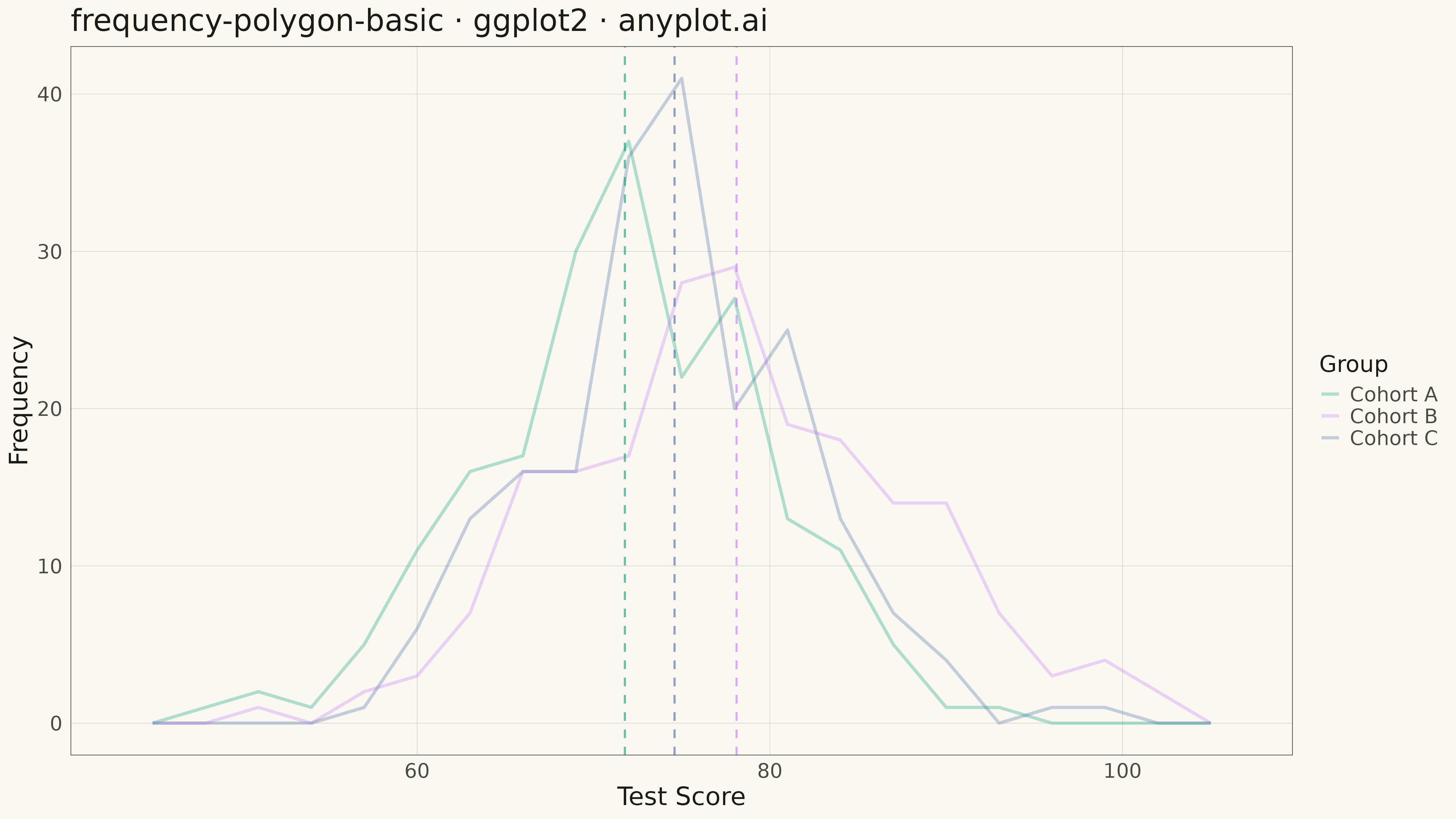
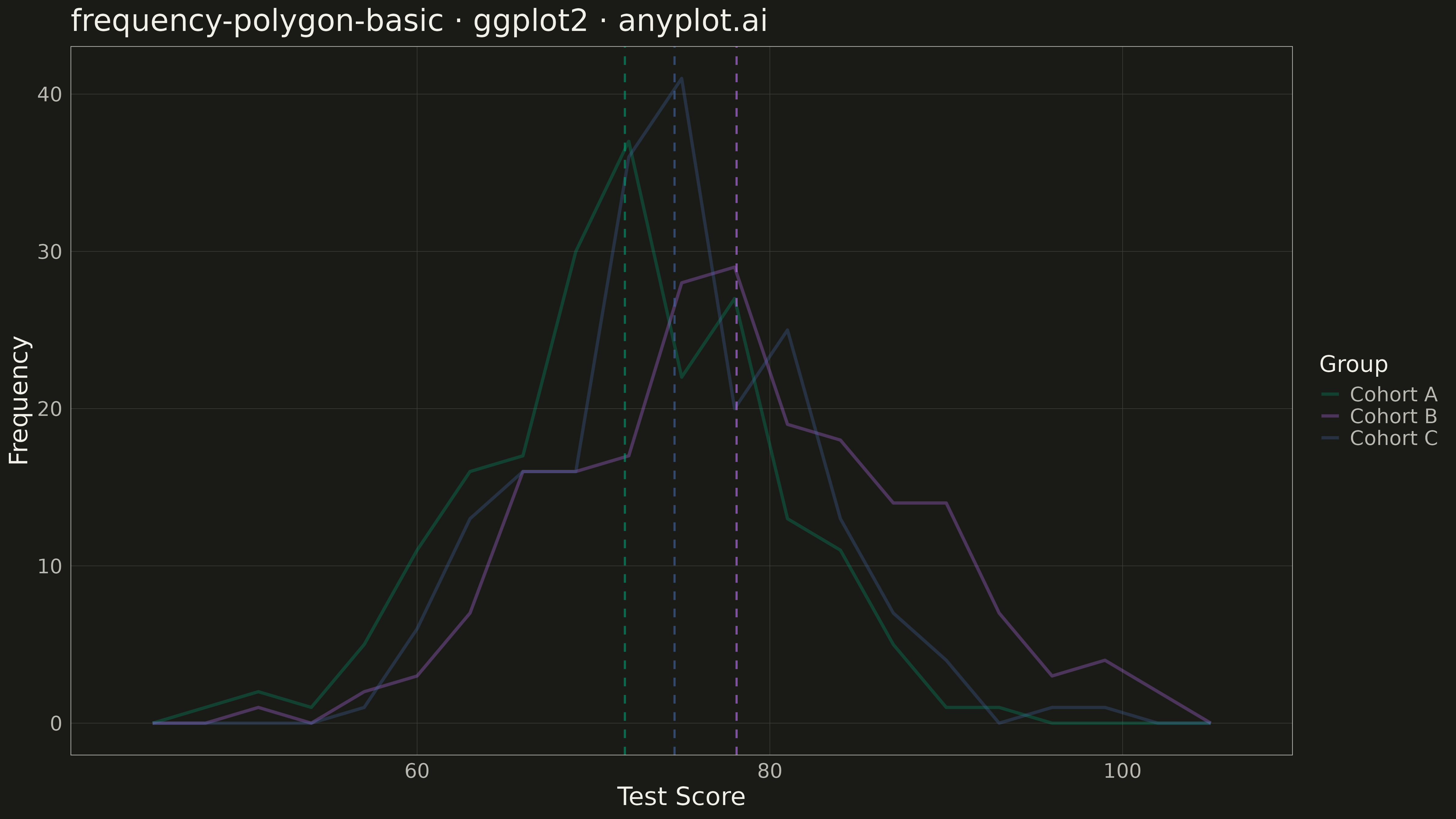
A frequency polygon connects the midpoints of histogram bins with straight line segments, creating an outline of the distribution shape. This visualization excels at comparing multiple distributions simultaneously since lines overlap without obscuring each other, unlike stacked or overlapping histogram bars. Frequency polygons reveal differences in central tendency, spread, skewness, and modality across groups with minimal visual clutter.
#' anyplot.ai
#' frequency-polygon-basic: Frequency Polygon for Distribution Comparison
#' Library: ggplot2 3.5.1 | R 4.4.1
#' Quality: 86/100 | Created: 2026-05-17

library(ggplot2)
library(ragg)

set.seed(42)

# --- Theme tokens -----------------------------------------------------------
THEME       <- Sys.getenv("ANYPLOT_THEME", "light")
PAGE_BG     <- if (THEME == "light") "#FAF8F1" else "#1A1A17"
INK         <- if (THEME == "light") "#1A1A17" else "#F0EFE8"
INK_SOFT    <- if (THEME == "light") "#4A4A44" else "#B8B7B0"
IMPRINT   <- c("#009E73", "#C475FD", "#4467A3", "#BD8233",
                 "#AE3030", "#2ABCCD", "#954477")

# --- Data -------------------------------------------------------------------
df <- data.frame(
  score = c(
    rnorm(200, mean = 72, sd = 8),   # Group A
    rnorm(200, mean = 78, sd = 10),  # Group B
    rnorm(200, mean = 75, sd = 7)    # Group C
  ),
  group = rep(c("Cohort A", "Cohort B", "Cohort C"), each = 200)
)

# --- Calculate group means for reference lines ---
group_means <- aggregate(score ~ group, data = df, FUN = mean)

# --- Plot -------------------------------------------------------------------
p <- ggplot(df, aes(x = score, color = group, fill = group)) +
  geom_freqpoly(binwidth = 3, linewidth = 1.2, alpha = 0.3) +
  geom_vline(
    data = group_means,
    aes(xintercept = score, color = group),
    linetype = "dashed",
    linewidth = 0.8,
    alpha = 0.6,
    show.legend = FALSE
  ) +
  scale_color_manual(values = IMPRINT[1:3]) +
  scale_fill_manual(values = IMPRINT[1:3]) +
  labs(
    title = "frequency-polygon-basic · ggplot2 · anyplot.ai",
    x = "Test Score",
    y = "Frequency",
    color = "Group",
    fill = "Group"
  ) +
  theme_minimal(base_size = 14) +
  theme(
    plot.background   = element_rect(fill = PAGE_BG, color = PAGE_BG),
    panel.background  = element_rect(fill = PAGE_BG, color = NA),
    panel.border      = element_rect(color = INK_SOFT, fill = NA, linewidth = 0.5),
    panel.grid.major  = element_line(color = if (THEME == "light") "#D0CECA" else "#3D3D39", linewidth = 0.2),
    panel.grid.minor  = element_blank(),
    axis.title        = element_text(color = INK, size = 20),
    axis.text         = element_text(color = INK_SOFT, size = 16),
    plot.title        = element_text(color = INK, size = 24),
    legend.background = element_rect(fill = PAGE_BG, color = NA),
    legend.text       = element_text(color = INK_SOFT, size = 16),
    legend.title      = element_text(color = INK, size = 18)
  )

# --- Save -------------------------------------------------------------------
ggsave(
  filename = sprintf("plot-%s.png", THEME),
  plot     = p,
  device   = ragg::agg_png,
  width    = 16,
  height   = 9,
  units    = "in",
  dpi      = 300
)
Runnable source as JSON, for any HTTP client: https://api.anyplot.ai/specs/frequency-polygon-basic/ggplot2/code. Any spec id and library id listed in llms-full.txt fit the same URL shape; every URL below is complete and callable.
{
  "spec_id": "frequency-polygon-basic",
  "language": "r",
  "library": "ggplot2",
  "page": "https://anyplot.ai/frequency-polygon-basic/r/ggplot2",
  "hub": "https://anyplot.ai/frequency-polygon-basic",
  "code_json": "https://api.anyplot.ai/specs/frequency-polygon-basic/ggplot2/code",
  "spec_json": "https://api.anyplot.ai/specs/frequency-polygon-basic",
  "render_light_png": "https://storage.googleapis.com/anyplot-images/plots/frequency-polygon-basic/r/ggplot2/plot-light.png",
  "render_dark_png": "https://storage.googleapis.com/anyplot-images/plots/frequency-polygon-basic/r/ggplot2/plot-dark.png",
  "quality_score": 86.0,
  "license": "MIT",
  "guide": "https://anyplot.ai/llms.txt"
}
Part of Frequency Polygon for Distribution Comparison on anyplot.ai.