The same plot in 14 other libraries — Python: Altair, Bokeh, lets-plot, Matplotlib, Plotly, plotnine, Pygal, Seaborn; Julia: Makie.jl; JavaScript: Chart.js, D3.js, Apache ECharts, Highcharts, MUI X Charts. Compare all 15 side by side: Ichimoku Cloud Technical Indicator Chart in Python, R, Julia and JavaScript.
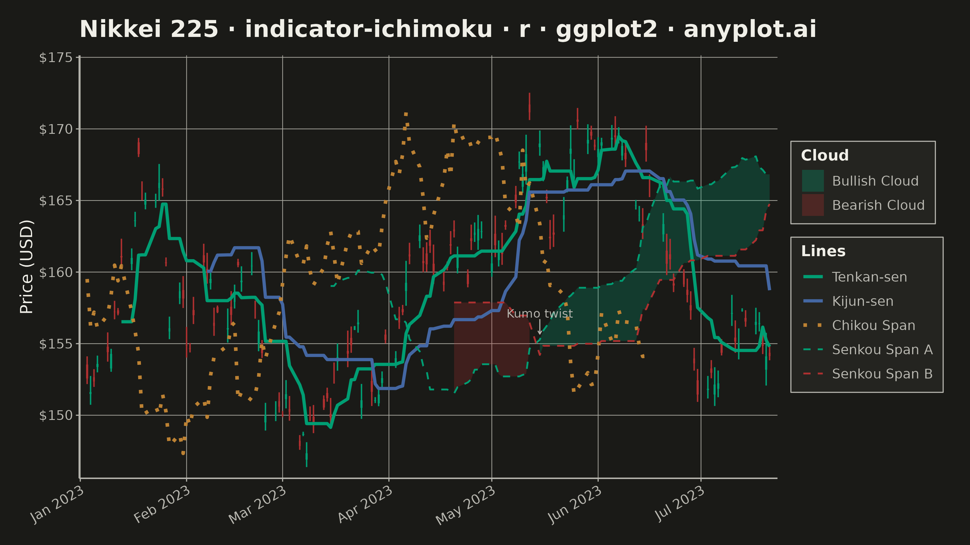
Displays the Ichimoku Kinko Hyo ("one glance equilibrium chart") overlay on a candlestick price chart. The indicator plots five lines — Tenkan-sen (conversion), Kijun-sen (base), Senkou Span A, Senkou Span B, and Chikou Span (lagging) — with the area between Senkou Span A and B filled as the "Kumo" (cloud). The cloud color changes depending on which span is on top, providing an at-a-glance view of trend direction, momentum, and support/resistance zones.
#' anyplot.ai
#' indicator-ichimoku: Ichimoku Cloud Technical Indicator Chart
#' Library: ggplot2 3.5.1 | R 4.4.1
#' Quality: 88/100 | Created: 2026-06-08

library(ggplot2)
library(dplyr)
library(tidyr)
library(scales)
library(ragg)

set.seed(42)

# Theme tokens
THEME       <- Sys.getenv("ANYPLOT_THEME", "light")
PAGE_BG     <- if (THEME == "light") "#FAF8F1" else "#1A1A17"
ELEVATED_BG <- if (THEME == "light") "#FFFDF6" else "#242420"
INK         <- if (THEME == "light") "#1A1A17" else "#F0EFE8"
INK_SOFT    <- if (THEME == "light") "#4A4A44" else "#B8B7B0"
INK_MUTED   <- if (THEME == "light") "#6B6A63" else "#A8A79F"

# Imprint palette
IMPRINT_PALETTE <- c(
    "#009E73",  # 1 — brand green
    "#C475FD",  # 2 — lavender
    "#4467A3",  # 3 — blue
    "#BD8233",  # 4 — ochre
    "#AE3030",  # 5 — matte red
    "#2ABCCD",  # 6 — cyan
    "#954477",  # 7 — rose
    "#99B314"   # 8 — lime
)

# Data — synthetic Nikkei 225 daily OHLC, ~160 trading days
n_periods <- 200
dates     <- seq.Date(as.Date("2023-01-03"), by = "day", length.out = n_periods)
dates     <- dates[weekdays(dates) %in% c("Monday", "Tuesday", "Wednesday", "Thursday", "Friday")]
dates     <- dates[seq_len(min(160, length(dates)))]
n         <- length(dates)

log_returns  <- cumsum(rnorm(n, mean = 0.0005, sd = 0.012))
close_prices <- 150 * exp(log_returns)
daily_range  <- abs(rnorm(n, mean = 0.008, sd = 0.004)) * close_prices
open_prices  <- close_prices - rnorm(n, 0, 0.003) * close_prices
high_prices  <- pmax(open_prices, close_prices) + daily_range * 0.6
low_prices   <- pmin(open_prices, close_prices) - daily_range * 0.4

# Ichimoku helpers (standard 9 / 26 / 52 parameters)
roll_high <- function(x, k) {
    sapply(seq_along(x), function(i) if (i < k) NA else max(x[(i - k + 1):i]))
}
roll_low <- function(x, k) {
    sapply(seq_along(x), function(i) if (i < k) NA else min(x[(i - k + 1):i]))
}

tenkan_sen    <- (roll_high(high_prices, 9)  + roll_low(low_prices, 9))  / 2
kijun_sen     <- (roll_high(high_prices, 26) + roll_low(low_prices, 26)) / 2
span_a_raw    <- (tenkan_sen + kijun_sen) / 2
span_b_raw    <- (roll_high(high_prices, 52) + roll_low(low_prices, 52)) / 2
senkou_span_a <- c(rep(NA, 26), span_a_raw)[seq_len(n)]
senkou_span_b <- c(rep(NA, 26), span_b_raw)[seq_len(n)]
chikou_span   <- c(close_prices[27:n], rep(NA, 26))

df <- data.frame(
    date          = dates,
    open          = open_prices,
    high          = high_prices,
    low           = low_prices,
    close         = close_prices,
    tenkan_sen    = tenkan_sen,
    kijun_sen     = kijun_sen,
    senkou_span_a = senkou_span_a,
    senkou_span_b = senkou_span_b,
    chikou_span   = chikou_span
)

df$up     <- df$close >= df$open
df$up_chr <- as.character(df$up)  # "TRUE"/"FALSE" strings for color scale

CANDLE_UP   <- IMPRINT_PALETTE[1]
CANDLE_DOWN <- IMPRINT_PALETTE[5]

# Cloud data split by bullish/bearish for two-color fill
df_cloud <- df |>
    filter(!is.na(senkou_span_a) & !is.na(senkou_span_b)) |>
    mutate(
        upper      = pmax(senkou_span_a, senkou_span_b),
        lower      = pmin(senkou_span_a, senkou_span_b),
        cloud_type = if_else(senkou_span_a >= senkou_span_b, "Bullish Cloud", "Bearish Cloud")
    )

# Indicator lines in long format — enables merged color+linetype legend
df_lines <- df |>
    pivot_longer(
        cols      = c(tenkan_sen, kijun_sen, chikou_span, senkou_span_a, senkou_span_b),
        names_to  = "indicator",
        values_to = "value"
    ) |>
    mutate(
        indicator = factor(
            indicator,
            levels = c("tenkan_sen", "kijun_sen", "chikou_span", "senkou_span_a", "senkou_span_b"),
            labels = c("Tenkan-sen", "Kijun-sen", "Chikou Span", "Senkou Span A", "Senkou Span B")
        )
    )

# Scale definitions
IND_BREAKS <- c("Tenkan-sen", "Kijun-sen", "Chikou Span", "Senkou Span A", "Senkou Span B")

# Combined color: candle wicks ("TRUE"/"FALSE") + indicator lines — wicks hidden via breaks
ALL_COLORS <- c(
    "TRUE"          = CANDLE_UP,
    "FALSE"         = CANDLE_DOWN,
    "Tenkan-sen"    = IMPRINT_PALETTE[1],
    "Kijun-sen"     = IMPRINT_PALETTE[3],
    "Chikou Span"   = IMPRINT_PALETTE[4],
    "Senkou Span A" = IMPRINT_PALETTE[1],
    "Senkou Span B" = IMPRINT_PALETTE[5]
)

# Combined fill: candle bodies + cloud — bodies hidden via breaks
ALL_FILLS <- c(
    "TRUE"          = CANDLE_UP,
    "FALSE"         = CANDLE_DOWN,
    "Bullish Cloud" = IMPRINT_PALETTE[1],
    "Bearish Cloud" = IMPRINT_PALETTE[5]
)

LINE_TYPES <- c(
    "Tenkan-sen"    = "solid",
    "Kijun-sen"     = "solid",
    "Chikou Span"   = "dotted",
    "Senkou Span A" = "dashed",
    "Senkou Span B" = "dashed"
)

# Find first Kumo twist (cloud color flip) for annotation
cloud_flips <- df_cloud |>
    arrange(date) |>
    mutate(prev_type = lag(cloud_type)) |>
    filter(!is.na(prev_type), cloud_type != prev_type)

# Title
title_str   <- "Nikkei 225 · indicator-ichimoku · r · ggplot2 · anyplot.ai"
n_title     <- nchar(title_str)
title_fs    <- max(8, round(12 * 67 / n_title))
price_range <- range(df$low, df$high, na.rm = TRUE)

p <- ggplot(df, aes(x = date)) +

    # Kumo (cloud) — bearish layer first, bullish on top; fill → Cloud legend
    geom_ribbon(
        data  = filter(df_cloud, cloud_type == "Bearish Cloud"),
        aes(ymin = lower, ymax = upper, fill = cloud_type),
        alpha = 0.25
    ) +
    geom_ribbon(
        data  = filter(df_cloud, cloud_type == "Bullish Cloud"),
        aes(ymin = lower, ymax = upper, fill = cloud_type),
        alpha = 0.25
    ) +

    # Candlestick wicks — color mapped for correct coloring, excluded from legend
    geom_segment(
        aes(xend = date, y = low, yend = high, color = up_chr),
        linewidth = 0.4
    ) +

    # Candlestick bodies — fill mapped for correct coloring, excluded from legend
    geom_rect(
        aes(
            xmin = date - 0.3, xmax = date + 0.3,
            ymin = pmin(open, close), ymax = pmax(open, close),
            fill = up_chr
        ),
        color = NA
    ) +

    # Tenkan-sen + Kijun-sen (thick solid momentum lines)
    geom_line(
        data      = filter(df_lines, indicator %in% c("Tenkan-sen", "Kijun-sen")),
        aes(y = value, color = indicator, linetype = indicator),
        linewidth = 0.9, na.rm = TRUE
    ) +
    # Chikou Span — thicker dotted line for visibility through candlestick forest
    geom_line(
        data      = filter(df_lines, indicator == "Chikou Span"),
        aes(y = value, color = indicator, linetype = indicator),
        linewidth = 1.0, na.rm = TRUE
    ) +
    # Senkou Span A + B (thin dashed cloud boundaries)
    geom_line(
        data      = filter(df_lines, indicator %in% c("Senkou Span A", "Senkou Span B")),
        aes(y = value, color = indicator, linetype = indicator),
        linewidth = 0.5, na.rm = TRUE
    ) +

    # Color scale: only indicator lines appear in "Lines" legend
    scale_color_manual(
        name   = "Lines",
        values = ALL_COLORS,
        breaks = IND_BREAKS
    ) +
    # Fill scale: only cloud fills appear in "Cloud" legend
    scale_fill_manual(
        name   = "Cloud",
        values = ALL_FILLS,
        breaks = c("Bullish Cloud", "Bearish Cloud")
    ) +
    # Linetype scale merged with color into one "Lines" legend box
    scale_linetype_manual(
        name   = "Lines",
        values = LINE_TYPES,
        breaks = IND_BREAKS
    ) +

    scale_x_date(
        date_breaks = "1 month",
        date_labels = "%b %Y",
        expand      = expansion(mult = 0.01)
    ) +
    scale_y_continuous(
        labels = label_dollar(),
        expand = expansion(mult = c(0.03, 0.10))
    ) +

    # Cloud legend keys show semi-transparent swatches (no border)
    guides(fill = guide_legend(override.aes = list(alpha = 0.3, color = NA))) +

    labs(
        title = title_str,
        x     = NULL,
        y     = "Price (USD)"
    ) +

    theme_minimal(base_size = 8) +
    theme(
        plot.background   = element_rect(fill = PAGE_BG,    color = PAGE_BG),
        panel.background  = element_rect(fill = PAGE_BG,    color = NA),
        panel.grid.major  = element_line(color = INK_MUTED, linewidth = 0.2),
        panel.grid.minor  = element_blank(),
        panel.border      = element_blank(),
        axis.title.y      = element_text(color = INK,      size = 10),
        axis.text         = element_text(color = INK_SOFT, size = 8),
        axis.text.x       = element_text(angle = 30, hjust = 1),
        axis.line         = element_line(color = INK_SOFT, linewidth = 0.4),
        axis.ticks        = element_line(color = INK_SOFT, linewidth = 0.3),
        plot.title        = element_text(color = INK, size = title_fs, face = "bold",
                                         margin = margin(b = 8)),
        plot.margin       = margin(12, 16, 10, 12),
        legend.background = element_rect(fill = ELEVATED_BG, color = INK_SOFT, linewidth = 0.3),
        legend.text       = element_text(color = INK_SOFT, size = 8),
        legend.title      = element_text(color = INK,      size = 9, face = "bold"),
        legend.key.size   = unit(1.0, "lines"),
        legend.position   = "right",
        legend.margin     = margin(4, 6, 4, 6)
    )

# Annotate first Kumo twist (cloud color flip = trend-change signal)
if (nrow(cloud_flips) > 0) {
    flip_date  <- cloud_flips$date[1]
    flip_upper <- df_cloud |> filter(date == flip_date) |> pull(upper)
    if (length(flip_upper) == 1 && !is.na(flip_upper)) {
        rng      <- diff(price_range)
        annot_y  <- flip_upper + rng * 0.07
        arrow_y1 <- annot_y   - rng * 0.015
        arrow_y2 <- flip_upper + rng * 0.015
        p <- p +
            annotate("text",
                     x = flip_date, y = annot_y,
                     label = "Kumo twist", color = INK_SOFT,
                     size = 2.5, hjust = 0.5) +
            annotate("segment",
                     x = flip_date, xend = flip_date,
                     y = arrow_y1, yend = arrow_y2,
                     color = INK_SOFT, linewidth = 0.3,
                     arrow = arrow(length = unit(0.08, "cm"), type = "open"))
    }
}

ggsave(
    filename = sprintf("plot-%s.png", THEME),
    plot     = p,
    device   = ragg::agg_png,
    width    = 8,
    height   = 4.5,
    units    = "in",
    dpi      = 400
)
Runnable source as JSON, for any HTTP client: https://api.anyplot.ai/specs/indicator-ichimoku/ggplot2/code. Any spec id and library id listed in llms-full.txt fit the same URL shape; every URL below is complete and callable.
{
  "spec_id": "indicator-ichimoku",
  "language": "r",
  "library": "ggplot2",
  "page": "https://anyplot.ai/indicator-ichimoku/r/ggplot2",
  "hub": "https://anyplot.ai/indicator-ichimoku",
  "code_json": "https://api.anyplot.ai/specs/indicator-ichimoku/ggplot2/code",
  "spec_json": "https://api.anyplot.ai/specs/indicator-ichimoku",
  "render_light_png": "https://storage.googleapis.com/anyplot-images/plots/indicator-ichimoku/r/ggplot2/plot-light.png",
  "render_dark_png": "https://storage.googleapis.com/anyplot-images/plots/indicator-ichimoku/r/ggplot2/plot-dark.png",
  "quality_score": 88.0,
  "license": "MIT",
  "guide": "https://anyplot.ai/llms.txt"
}
Part of Ichimoku Cloud Technical Indicator Chart on anyplot.ai.