The same plot in 14 other libraries — JavaScript: Chart.js, Apache ECharts, Highcharts, MUI X Charts; Python: Altair, Bokeh, lets-plot, Matplotlib, Plotly, plotnine, Pygal, Seaborn; R: ggplot2; Julia: Makie.jl. Compare all 15 side by side: Gini Impurity vs Entropy Comparison in Python, R, Julia and JavaScript.
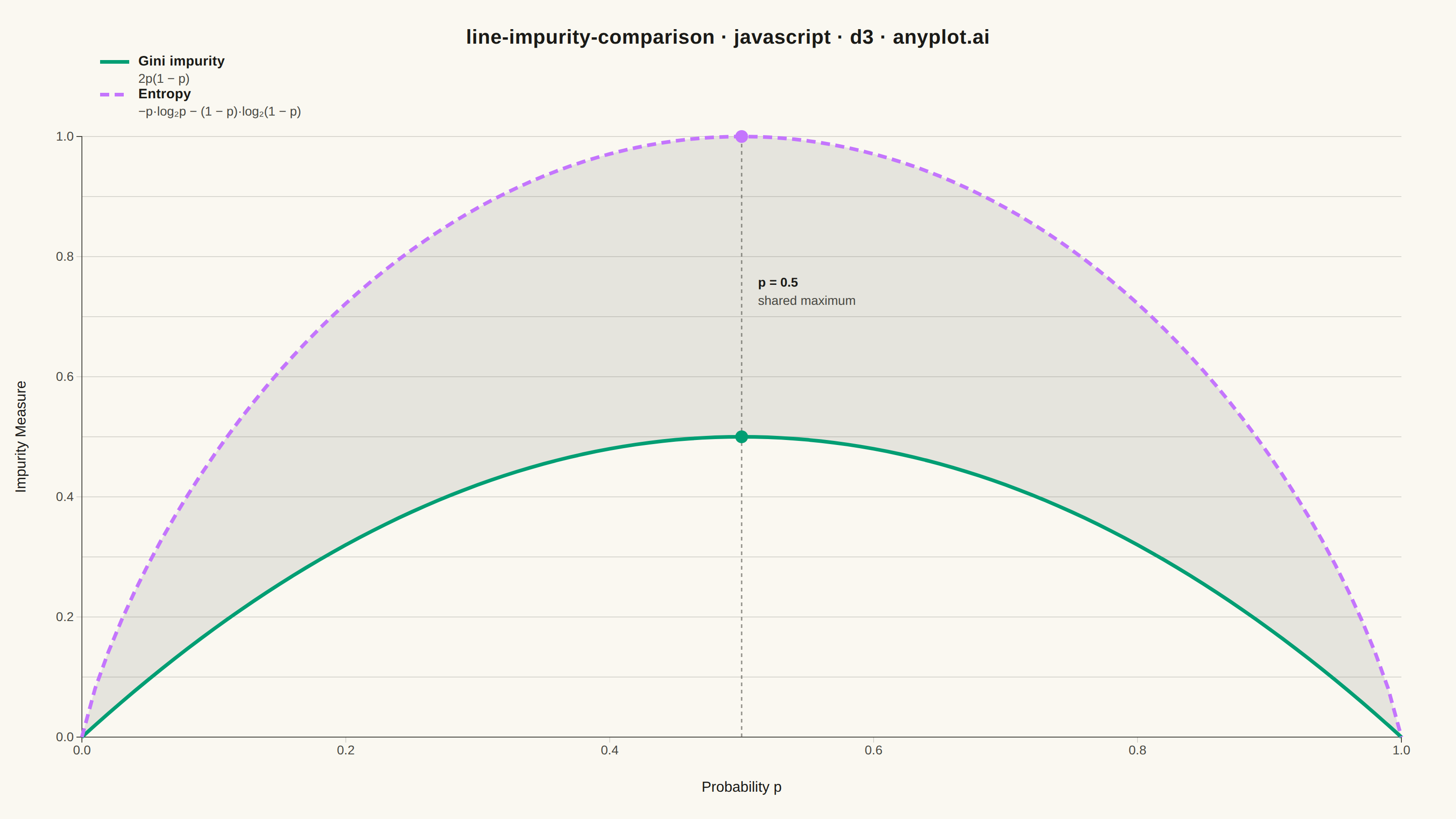
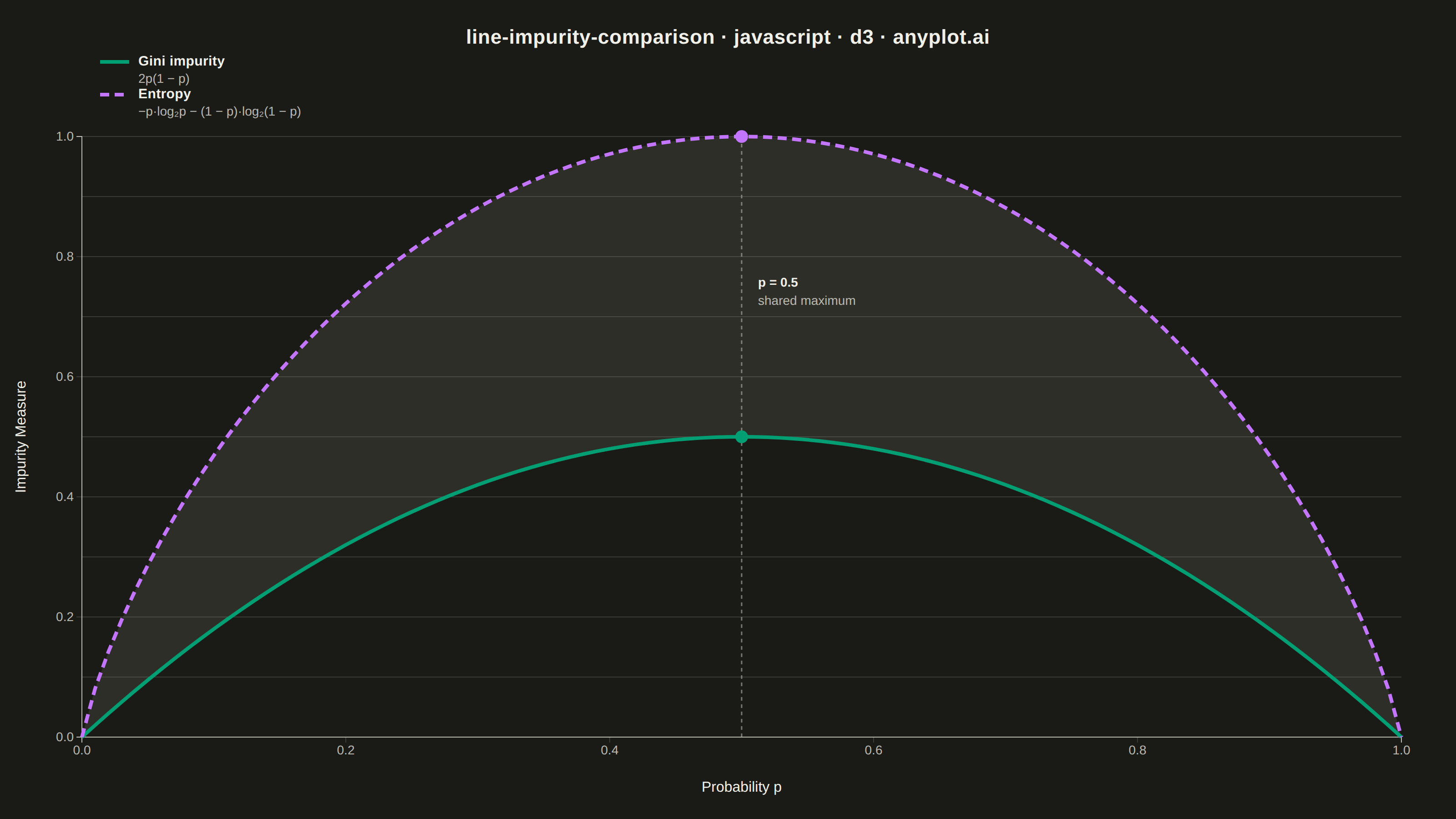
A theoretical comparison plot showing Gini impurity and entropy (information gain) as splitting criteria for decision trees across the probability range [0, 1]. Both curves are displayed on the same axes to illustrate their similar behavior and slight differences. This educational visualization helps understand the mathematical foundation of tree-based algorithms and why both criteria lead to similar tree structures in practice.
// anyplot.ai
// line-impurity-comparison: Gini Impurity vs Entropy Comparison
// Library: d3 7.9.0 | JavaScript 22.23.2
// Quality: 94/100 | Created: 2026-08-26

//# anyplot-orientation: landscape
const t = window.ANYPLOT_TOKENS;
const { width, height } = window.ANYPLOT_SIZE;
const margin = { top: 150, right: 60, bottom: 90, left: 90 };
const iw = width - margin.left - margin.right;
const ih = height - margin.top - margin.bottom;

// --- Data (in-memory, deterministic) ----------------------------------------
// Gini impurity: 2p(1-p). Entropy (log2, normalized): -p*log2(p) - (1-p)*log2(1-p).
const gini = (p) => 2 * p * (1 - p);
const entropy = (p) => (p === 0 || p === 1 ? 0 : -p * Math.log2(p) - (1 - p) * Math.log2(1 - p));

const probabilities = d3.range(0, 101).map((i) => i / 100);
const giniCurve = probabilities.map((p) => ({ p, value: gini(p) }));
const entropyCurve = probabilities.map((p) => ({ p, value: entropy(p) }));
// Entropy >= Gini across the whole domain, so a single area band between the
// two curves is well-defined (no crossing) and reads as "how closely they track".
const trackBand = probabilities.map((p) => ({ p, lo: gini(p), hi: entropy(p) }));

const muted = window.ANYPLOT_THEME === "dark" ? "#A8A79F" : "#6B6A63";

// --- SVG mount ----------------------------------------------------------------
const svg = d3.select("#container").append("svg").attr("width", width).attr("height", height);
const g = svg.append("g").attr("transform", `translate(${margin.left},${margin.top})`);

// --- Scales ---------------------------------------------------------------
const x = d3.scaleLinear().domain([0, 1]).range([0, iw]);
const y = d3.scaleLinear().domain([0, 1]).nice().range([ih, 0]);

// --- Grid (light, y-axis only) ---------------------------------------------
g.append("g")
  .attr("class", "grid")
  .call(d3.axisLeft(y).tickSize(-iw).tickFormat(""))
  .call((sel) => sel.select(".domain").remove())
  .selectAll("line")
  .attr("stroke", t.grid);

// --- Axes -------------------------------------------------------------------
const xAxis = g
  .append("g")
  .attr("transform", `translate(0,${ih})`)
  .call(d3.axisBottom(x).ticks(6));
const yAxis = g.append("g").call(d3.axisLeft(y).ticks(6));
for (const ax of [xAxis, yAxis]) {
  ax.selectAll("text").attr("fill", t.inkSoft).style("font-size", "14px");
  ax.selectAll("line").attr("stroke", t.grid);
  ax.select(".domain").attr("stroke", t.inkSoft);
}

// --- Axis labels --------------------------------------------------------------
g.append("text")
  .attr("x", iw / 2)
  .attr("y", ih + 60)
  .attr("text-anchor", "middle")
  .attr("fill", t.ink)
  .style("font-size", "16px")
  .text("Probability p");

g.append("text")
  .attr("transform", "rotate(-90)")
  .attr("x", -ih / 2)
  .attr("y", -62)
  .attr("text-anchor", "middle")
  .attr("fill", t.ink)
  .style("font-size", "16px")
  .text("Impurity Measure");

// --- Track band: fill between the curves (D3-distinctive d3.area) -------------
// Emphasizes the spec's core insight — Gini and Entropy track closely across
// the whole range, not just at their shared maximum.
const band = d3
  .area()
  .x((d) => x(d.p))
  .y0((d) => y(d.lo))
  .y1((d) => y(d.hi));

g.append("path").datum(trackBand).attr("fill", muted).attr("opacity", 0.14).attr("d", band);

// --- Lines --------------------------------------------------------------------
const line = d3
  .line()
  .x((d) => x(d.p))
  .y((d) => y(d.value));

g.append("path")
  .datum(giniCurve)
  .attr("fill", "none")
  .attr("stroke", t.palette[0])
  .attr("stroke-width", 4)
  .attr("d", line);

g.append("path")
  .datum(entropyCurve)
  .attr("fill", "none")
  .attr("stroke", t.palette[1])
  .attr("stroke-width", 4)
  .attr("stroke-dasharray", "10,6")
  .attr("d", line);

// --- Annotation: shared maximum at p=0.5 (spec-requested) ---------------------
const guideX = x(0.5);
g.append("line")
  .attr("x1", guideX)
  .attr("x2", guideX)
  .attr("y1", y(0))
  .attr("y2", y(1))
  .attr("stroke", t.inkSoft)
  .attr("stroke-width", 1.5)
  .attr("stroke-dasharray", "4,4")
  .attr("opacity", 0.6);

g.append("circle").attr("cx", guideX).attr("cy", y(gini(0.5))).attr("r", 7).attr("fill", t.palette[0]);
g.append("circle").attr("cx", guideX).attr("cy", y(entropy(0.5))).attr("r", 7).attr("fill", t.palette[1]);

// Label sits in the open gap between the two curves, clear of both lines.
// Two-tier typography: bold value line, lighter-weight caption line.
g.append("text")
  .attr("x", guideX + 18)
  .attr("y", y((gini(0.5) + entropy(0.5)) / 2))
  .attr("fill", t.ink)
  .style("font-size", "14px")
  .style("font-weight", "600")
  .text("p = 0.5")
  .append("tspan")
  .attr("x", guideX + 18)
  .attr("dy", 20)
  .attr("fill", t.inkSoft)
  .style("font-weight", "400")
  .text("shared maximum");

// --- Legend (with formulas) ----------------------------------------------------
const legend = svg
  .append("g")
  .attr("transform", `translate(${margin.left + 20},${margin.top - 78})`);

const legendRows = [
  { name: "Gini impurity", formula: "2p(1 − p)", color: t.palette[0], dash: null },
  { name: "Entropy", formula: "−p·log₂p − (1 − p)·log₂(1 − p)", color: t.palette[1], dash: "10,6" },
];

// Two-tier typography: bold metric name, lighter-weight formula beneath it —
// gives the legend a clearer hierarchy than a single undifferentiated line.
legendRows.forEach((d, i) => {
  const row = legend.append("g").attr("transform", `translate(0,${i * 36})`);
  row
    .append("line")
    .attr("x1", 0)
    .attr("x2", 32)
    .attr("y1", -4)
    .attr("y2", -4)
    .attr("stroke", d.color)
    .attr("stroke-width", 4)
    .attr("stroke-dasharray", d.dash);
  row
    .append("text")
    .attr("x", 42)
    .attr("y", 0)
    .attr("fill", t.ink)
    .style("font-size", "15px")
    .style("font-weight", "600")
    .style("letter-spacing", "0.2px")
    .text(d.name);
  row
    .append("text")
    .attr("x", 42)
    .attr("y", 19)
    .attr("fill", t.inkSoft)
    .style("font-size", "14px")
    .style("font-weight", "400")
    .text(d.formula);
});

// --- Title ----------------------------------------------------------------
svg
  .append("text")
  .attr("x", width / 2)
  .attr("y", 48)
  .attr("text-anchor", "middle")
  .attr("fill", t.ink)
  .style("font-size", "22px")
  .style("font-weight", "600")
  .style("letter-spacing", "0.4px")
  .text("line-impurity-comparison · javascript · d3 · anyplot.ai");
Runnable source as JSON, for any HTTP client: https://api.anyplot.ai/specs/line-impurity-comparison/d3/code. Any spec id and library id listed in llms-full.txt fit the same URL shape; every URL below is complete and callable.
{
  "spec_id": "line-impurity-comparison",
  "language": "javascript",
  "library": "d3",
  "page": "https://anyplot.ai/line-impurity-comparison/javascript/d3",
  "hub": "https://anyplot.ai/line-impurity-comparison",
  "code_json": "https://api.anyplot.ai/specs/line-impurity-comparison/d3/code",
  "spec_json": "https://api.anyplot.ai/specs/line-impurity-comparison",
  "render_light_png": "https://storage.googleapis.com/anyplot-images/plots/line-impurity-comparison/javascript/d3/plot-light.png",
  "render_dark_png": "https://storage.googleapis.com/anyplot-images/plots/line-impurity-comparison/javascript/d3/plot-dark.png",
  "interactive_light_html": "https://storage.googleapis.com/anyplot-images/plots/line-impurity-comparison/javascript/d3/plot-light.html",
  "interactive_dark_html": "https://storage.googleapis.com/anyplot-images/plots/line-impurity-comparison/javascript/d3/plot-dark.html",
  "quality_score": 94.0,
  "license": "MIT",
  "guide": "https://anyplot.ai/llms.txt"
}
Part of Gini Impurity vs Entropy Comparison on anyplot.ai.