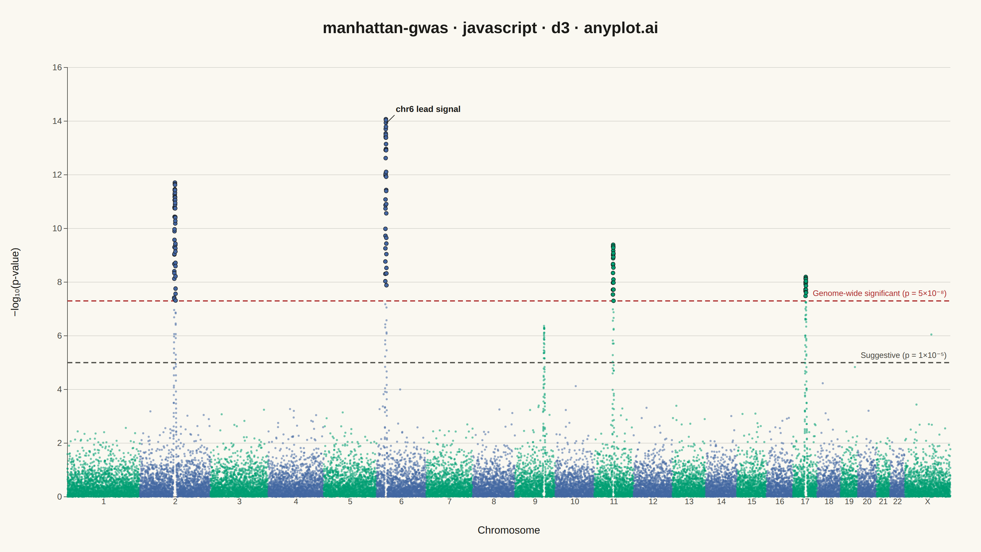
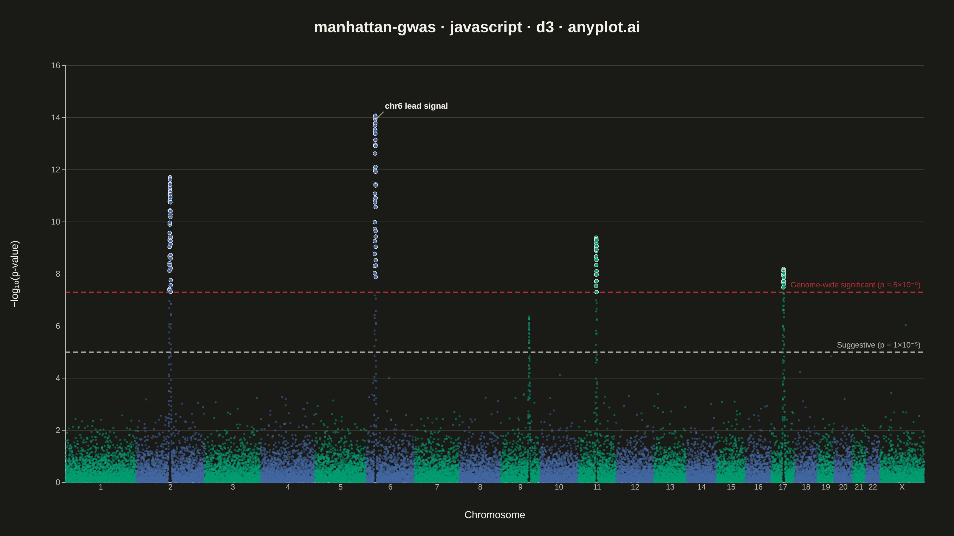
The same plot in 14 other libraries — JavaScript: Chart.js, Apache ECharts, Highcharts, MUI X Charts; Python: Altair, Bokeh, lets-plot, Matplotlib, Plotly, plotnine, Pygal, Seaborn; R: ggplot2; Julia: Makie.jl. Compare all 15 side by side: Manhattan Plot for GWAS in Python, R, Julia and JavaScript.
A Manhattan plot visualizes genome-wide association study (GWAS) results by displaying -log10 transformed p-values across chromosomal positions. Points are arranged by genomic position along the x-axis with alternating colors for each chromosome, making it easy to identify significant associations. A horizontal threshold line indicates genome-wide significance (typically p < 5×10⁻⁸). This plot is essential for identifying genetic variants associated with traits or diseases.
// anyplot.ai
// manhattan-gwas: Manhattan Plot for GWAS
// Library: d3 7.9.0 | JavaScript 22.23.2
// Quality: 93/100 | Created: 2026-09-05

const t = window.ANYPLOT_TOKENS;
const { width, height } = window.ANYPLOT_SIZE;
const margin = { top: 110, right: 50, bottom: 90, left: 110 };
const iw = width - margin.left - margin.right;
const ih = height - margin.top - margin.bottom;

// --- Deterministic PRNG (LCG) ------------------------------------------------
function makeLcg(seed) {
  let state = seed;
  return () => {
    state = (state * 1664525 + 1013904223) % 4294967296;
    return state / 4294967296;
  };
}
const rng = makeLcg(42);

// --- Data: simulated GWAS scan across 22 autosomes + X (approx. GRCh38 Mb) --
const chromLengthsMb = {
  "1": 248.9, "2": 242.2, "3": 198.3, "4": 190.2, "5": 181.5, "6": 170.8,
  "7": 159.3, "8": 145.1, "9": 138.4, "10": 133.8, "11": 135.1, "12": 133.3,
  "13": 114.4, "14": 107.0, "15": 101.9, "16": 90.3, "17": 83.3, "18": 80.4,
  "19": 58.6, "20": 64.4, "21": 46.7, "22": 50.8, "X": 156.0,
};
const chromosomes = Object.keys(chromLengthsMb);
const pointsPerMb = 10;

// Localized association peaks (linkage-disequilibrium-like bumps above the null background)
const peaks = [
  { chrom: "2", posMb: 120, height: 11.5, width: 2.5 },
  { chrom: "6", posMb: 32, height: 13.8, width: 1.8 },
  { chrom: "9", posMb: 100, height: 6.2, width: 2.0 },
  { chrom: "11", posMb: 65, height: 9.4, width: 1.5 },
  { chrom: "17", posMb: 44, height: 8.0, width: 2.2 },
];

const chromOffsetMb = {};
let cumulativeMb = 0;
const data = [];
for (const chrom of chromosomes) {
  chromOffsetMb[chrom] = cumulativeMb;
  const lengthMb = chromLengthsMb[chrom];
  const n = Math.round(lengthMb * pointsPerMb);
  for (let i = 0; i < n; i++) {
    const posMb = ((i + rng()) / n) * lengthMb;

    // Null-model background: -log10(p) for p ~ Uniform(0, 1)
    let negLogP = -Math.log10(rng());

    // Overlay any peak centered on this chromosome
    for (const peak of peaks) {
      if (peak.chrom !== chrom) continue;
      const d = posMb - peak.posMb;
      const bump = peak.height * Math.exp(-(d * d) / (2 * peak.width * peak.width));
      if (bump > negLogP) negLogP = bump + (rng() - 0.5) * 0.6;
    }

    data.push({ chrom, cumPos: cumulativeMb + posMb, negLogP: Math.max(0, negLogP) });
  }
  cumulativeMb += lengthMb;
}
const genomeLengthMb = cumulativeMb;
const genomeWideThreshold = -Math.log10(5e-8); // ~7.3
const suggestiveThreshold = -Math.log10(1e-5); // 5

// --- SVG mount ----------------------------------------------------------------
const svg = d3.select("#container").append("svg").attr("width", width).attr("height", height);
const g = svg.append("g").attr("transform", `translate(${margin.left},${margin.top})`);

// --- Scales ---------------------------------------------------------------
const x = d3.scaleLinear().domain([0, genomeLengthMb]).range([0, iw]);
const y = d3
  .scaleLinear()
  .domain([0, d3.max(data, (d) => d.negLogP) + 1])
  .nice()
  .range([ih, 0]);
const color = d3.scaleOrdinal().domain(chromosomes).range([t.palette[0], t.palette[2]]);

// --- Y grid + axis ----------------------------------------------------------
g.append("g")
  .attr("class", "grid")
  .call(d3.axisLeft(y).tickSize(-iw).tickFormat(""))
  .call((sel) => sel.select(".domain").remove())
  .selectAll("line")
  .attr("stroke", t.grid);

const yAxis = g.append("g").call(d3.axisLeft(y).ticks(6));
yAxis.selectAll("text").attr("fill", t.inkSoft).style("font-size", "14px");
yAxis.selectAll("line").attr("stroke", t.inkSoft);
yAxis.select(".domain").attr("stroke", t.inkSoft);

g.append("text")
  .attr("transform", "rotate(-90)")
  .attr("x", -ih / 2)
  .attr("y", -80)
  .attr("text-anchor", "middle")
  .attr("fill", t.ink)
  .style("font-size", "17px")
  .text("−log₁₀(p-value)");

// --- X axis: chromosome labels centered on each chromosome region -----------
const xAxis = g
  .append("g")
  .attr("transform", `translate(0,${ih})`)
  .call(
    d3
      .axisBottom(x)
      .tickValues(chromosomes.map((c) => chromOffsetMb[c] + chromLengthsMb[c] / 2))
      .tickFormat((_, i) => chromosomes[i])
      .tickSize(0)
  );
xAxis.selectAll("text").attr("fill", t.inkSoft).style("font-size", "13px");
xAxis.select(".domain").attr("stroke", t.inkSoft);

g.append("text")
  .attr("x", iw / 2)
  .attr("y", ih + 60)
  .attr("text-anchor", "middle")
  .attr("fill", t.ink)
  .style("font-size", "17px")
  .text("Chromosome");

// --- Significance threshold lines --------------------------------------------
function thresholdLine(value, label, stroke) {
  g.append("line")
    .attr("x1", 0)
    .attr("x2", iw)
    .attr("y1", y(value))
    .attr("y2", y(value))
    .attr("stroke", stroke)
    .attr("stroke-width", 2)
    .attr("stroke-dasharray", "8,5");
  g.append("text")
    .attr("x", iw - 6)
    .attr("y", y(value) - 8)
    .attr("text-anchor", "end")
    .attr("fill", stroke)
    .style("font-size", "13px")
    .text(label);
}
thresholdLine(suggestiveThreshold, "Suggestive (p = 1×10⁻⁵)", t.inkSoft);
thresholdLine(genomeWideThreshold, "Genome-wide significant (p = 5×10⁻⁸)", t.palette[4]);

// --- Points: alternating chromosome color, sized down for overplotting ------
g.selectAll("circle.point")
  .data(data)
  .join("circle")
  .attr("class", "point")
  .attr("cx", (d) => x(d.cumPos))
  .attr("cy", (d) => y(d.negLogP))
  .attr("r", 1.7)
  .attr("fill", (d) => color(d.chrom))
  .attr("opacity", 0.55);

// Genome-wide-significant SNPs get a bigger, outlined, fully opaque marker so
// they stand out from the null-distribution band instead of sharing its color only.
const significant = data.filter((d) => d.negLogP >= genomeWideThreshold);
g.selectAll("circle.significant")
  .data(significant)
  .join("circle")
  .attr("class", "significant")
  .attr("cx", (d) => x(d.cumPos))
  .attr("cy", (d) => y(d.negLogP))
  .attr("r", 3.2)
  .attr("fill", (d) => color(d.chrom))
  .attr("stroke", t.ink)
  .attr("stroke-width", 0.8)
  .attr("opacity", 1);

// --- Lead-signal callout: d3-quadtree nearest-neighbor lookup pinpoints the
// actual rendered point closest to the tallest peak's theoretical apex, so the
// annotation anchors to a real datum rather than an idealized coordinate -----
const pointIndex = d3.quadtree()
  .x((d) => x(d.cumPos))
  .y((d) => y(d.negLogP))
  .addAll(data);
const strongestPeak = peaks.reduce((a, b) => (b.height > a.height ? b : a));
const targetX = x(chromOffsetMb[strongestPeak.chrom] + strongestPeak.posMb);
const targetY = y(strongestPeak.height);
const leadSnp = pointIndex.find(targetX, targetY, 40);
if (leadSnp) {
  const ax = x(leadSnp.cumPos);
  const ay = y(leadSnp.negLogP);
  const labelX = ax + 16;
  const labelY = ay - 24;
  g.append("line")
    .attr("x1", ax)
    .attr("y1", ay - 5)
    .attr("x2", labelX - 2)
    .attr("y2", labelY + 5)
    .attr("stroke", t.ink)
    .attr("stroke-width", 1);
  g.append("text")
    .attr("x", labelX)
    .attr("y", labelY)
    .attr("text-anchor", "start")
    .attr("fill", t.ink)
    .style("font-size", "14px")
    .style("font-weight", "600")
    .text(`chr${leadSnp.chrom} lead signal`);
}

// --- Title --------------------------------------------------------------------
svg
  .append("text")
  .attr("x", width / 2)
  .attr("y", 54)
  .attr("text-anchor", "middle")
  .attr("fill", t.ink)
  .style("font-size", "26px")
  .style("font-weight", "600")
  .text("manhattan-gwas · javascript · d3 · anyplot.ai");
Runnable source as JSON, for any HTTP client: https://api.anyplot.ai/specs/manhattan-gwas/d3/code. Any spec id and library id listed in llms-full.txt fit the same URL shape; every URL below is complete and callable.
{
  "spec_id": "manhattan-gwas",
  "language": "javascript",
  "library": "d3",
  "page": "https://anyplot.ai/manhattan-gwas/javascript/d3",
  "hub": "https://anyplot.ai/manhattan-gwas",
  "code_json": "https://api.anyplot.ai/specs/manhattan-gwas/d3/code",
  "spec_json": "https://api.anyplot.ai/specs/manhattan-gwas",
  "render_light_png": "https://storage.googleapis.com/anyplot-images/plots/manhattan-gwas/javascript/d3/plot-light.png",
  "render_dark_png": "https://storage.googleapis.com/anyplot-images/plots/manhattan-gwas/javascript/d3/plot-dark.png",
  "interactive_light_html": "https://storage.googleapis.com/anyplot-images/plots/manhattan-gwas/javascript/d3/plot-light.html",
  "interactive_dark_html": "https://storage.googleapis.com/anyplot-images/plots/manhattan-gwas/javascript/d3/plot-dark.html",
  "quality_score": 93.0,
  "license": "MIT",
  "guide": "https://anyplot.ai/llms.txt"
}
Part of Manhattan Plot for GWAS on anyplot.ai.