The same plot in 14 other libraries — Python: Altair, Bokeh, lets-plot, Matplotlib, Plotly, plotnine, Pygal, Seaborn; Julia: Makie.jl; JavaScript: Chart.js, D3.js, Apache ECharts, Highcharts, MUI X Charts. Compare all 15 side by side: Manhattan Plot for GWAS in Python, R, Julia and JavaScript.
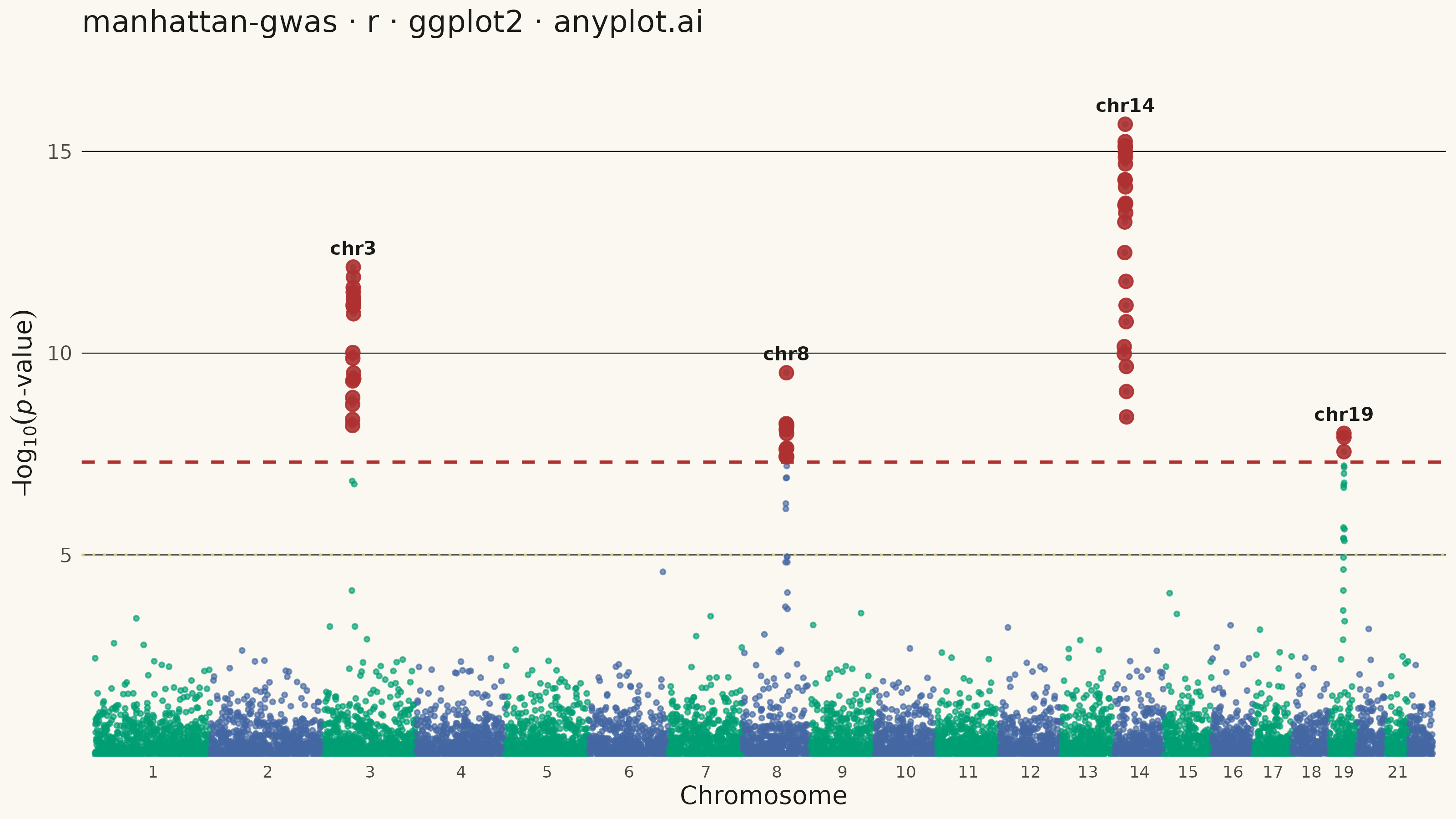
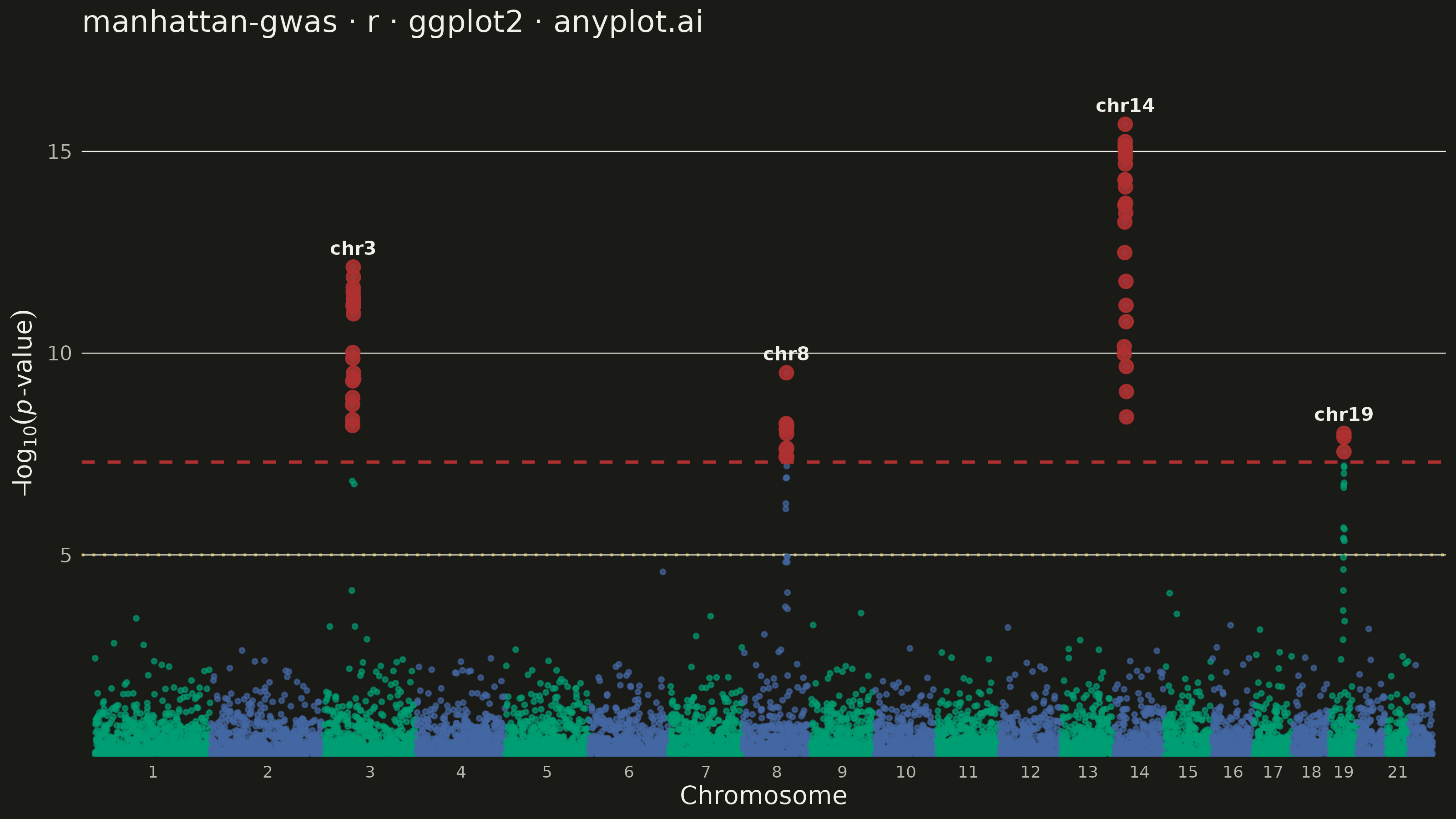
A Manhattan plot visualizes genome-wide association study (GWAS) results by displaying -log10 transformed p-values across chromosomal positions. Points are arranged by genomic position along the x-axis with alternating colors for each chromosome, making it easy to identify significant associations. A horizontal threshold line indicates genome-wide significance (typically p < 5×10⁻⁸). This plot is essential for identifying genetic variants associated with traits or diseases.
#' anyplot.ai
#' manhattan-gwas: Manhattan Plot for GWAS
#' Library: ggplot2 3.5.1 | R 4.4.1
#' Quality: 93/100 | Created: 2026-09-05

library(ggplot2)
library(dplyr)
library(ragg)

set.seed(42)

# --- Theme tokens -----------------------------------------------------------
THEME       <- Sys.getenv("ANYPLOT_THEME", "light")
PAGE_BG     <- if (THEME == "light") "#FAF8F1" else "#1A1A17"
INK         <- if (THEME == "light") "#1A1A17" else "#F0EFE8"
INK_SOFT    <- if (THEME == "light") "#4A4A44" else "#B8B7B0"
IMPRINT_PALETTE <- c("#009E73", "#C475FD", "#4467A3", "#BD8233",
                     "#AE3030", "#2ABCCD", "#954477", "#99B314")
ANYPLOT_AMBER <- "#DDCC77"

# --- Data --------------------------------------------------------------------
# Approximate human chromosome lengths (Mb), chromosomes 1-22
chr_lengths <- c(
  249, 243, 198, 191, 180, 171, 159, 145, 138, 133,
  135, 133, 114, 107, 102, 90, 83, 80, 59, 63, 48, 51
)
n_chr <- length(chr_lengths)

chr_info <- tibble::tibble(
  chromosome = 1:n_chr,
  length_mb  = chr_lengths
) %>%
  mutate(offset = lag(cumsum(length_mb), default = 0) * 1e6)

n_snps_total <- 9000
snps_per_chr <- round(n_snps_total * chr_lengths / sum(chr_lengths))

snps <- lapply(1:n_chr, function(i) {
  tibble::tibble(
    chromosome = i,
    position   = sort(sample(seq_len(chr_lengths[i] * 1e6), snps_per_chr[i])),
    p_value    = runif(snps_per_chr[i])
  )
}) %>% bind_rows()

# Simulated GWAS hits: clusters of low p-values around a few causal loci
peak_chr      <- c(3, 8, 14, 19)
peak_lead_log <- c(12.0, 9.2, 15.4, 7.8)
peaks <- Map(function(chr, lead_log) {
  cluster_size <- 24
  spread_bp    <- rnorm(cluster_size, 0, 1.5e6)
  lead_pos     <- sample(seq_len(chr_lengths[chr] * 1e6), 1)
  cluster_pos  <- pmin(pmax(lead_pos + spread_bp, 1), chr_lengths[chr] * 1e6)
  cluster_log  <- pmax(0.1, lead_log - abs(spread_bp) / 4e5 + rnorm(cluster_size, 0, 0.3))
  tibble::tibble(
    chromosome = chr,
    position   = round(cluster_pos),
    p_value    = 10^(-cluster_log)
  )
}, peak_chr, peak_lead_log) %>% bind_rows()

gwas <- bind_rows(snps, peaks) %>%
  left_join(chr_info, by = "chromosome") %>%
  mutate(
    bp_cum     = position + offset,
    neg_log_p  = -log10(p_value),
    chr_parity = ifelse(chromosome %% 2 == 0, "even", "odd")
  )

chr_axis <- chr_info %>%
  mutate(
    center = offset + length_mb * 1e6 / 2,
    # Chromosomes 19-22 are short and sit close together; thin the labels
    # past 18 to give the remaining ones breathing room.
    label  = ifelse(chromosome > 18 & chromosome %% 2 == 0, "", chromosome)
  )

genome_wide_line <- -log10(5e-8)
suggestive_line  <- -log10(1e-5)
sig_hits         <- gwas %>% filter(p_value < 5e-8)

# Lead SNP (highest -log10 p) per significant locus, for peak annotation
lead_snps <- sig_hits %>%
  group_by(chromosome) %>%
  slice_max(neg_log_p, n = 1, with_ties = FALSE) %>%
  ungroup()

# --- Plot ----------------------------------------------------------------
p <- ggplot(gwas, aes(x = bp_cum, y = neg_log_p, color = chr_parity)) +
  geom_hline(yintercept = suggestive_line, linetype = "dotted",
             color = ANYPLOT_AMBER, linewidth = 0.5) +
  geom_hline(yintercept = genome_wide_line, linetype = "dashed",
             color = IMPRINT_PALETTE[5], linewidth = 0.6) +
  geom_point(size = 0.6, alpha = 0.65) +
  geom_point(data = sig_hits, aes(x = bp_cum, y = neg_log_p),
             color = IMPRINT_PALETTE[5], size = 2.2, alpha = 0.9, inherit.aes = FALSE) +
  geom_text(data = lead_snps, aes(x = bp_cum, y = neg_log_p, label = paste0("chr", chromosome)),
            color = INK, size = 2.6, fontface = "bold", vjust = -0.9, inherit.aes = FALSE) +
  scale_color_manual(values = c(odd = IMPRINT_PALETTE[1], even = IMPRINT_PALETTE[3])) +
  scale_x_continuous(breaks = chr_axis$center, labels = chr_axis$label,
                      expand = expansion(mult = 0.01)) +
  scale_y_continuous(expand = expansion(mult = c(0, 0.12))) +
  labs(
    title = "manhattan-gwas · r · ggplot2 · anyplot.ai",
    x     = "Chromosome",
    y     = expression(-log[10](italic(p) * "-value"))
  ) +
  guides(color = "none") +
  theme_minimal(base_size = 8) +
  theme(
    plot.background   = element_rect(fill = PAGE_BG, color = PAGE_BG),
    panel.background  = element_rect(fill = PAGE_BG, color = NA),
    panel.grid.major.x = element_blank(),
    panel.grid.minor.x = element_blank(),
    panel.grid.minor.y = element_blank(),
    panel.grid.major.y = element_line(color = INK, linewidth = 0.2),
    axis.title        = element_text(color = INK, size = 10),
    axis.text.y       = element_text(color = INK_SOFT, size = 8),
    axis.text.x       = element_text(color = INK_SOFT, size = 6.5),
    plot.title        = element_text(color = INK, size = 12)
  )

# --- Save --------------------------------------------------------------------
ggsave(
  filename = sprintf("plot-%s.png", THEME),
  plot     = p,
  device   = ragg::agg_png,
  width    = 8,
  height   = 4.5,
  units    = "in",
  dpi      = 400
)
Runnable source as JSON, for any HTTP client: https://api.anyplot.ai/specs/manhattan-gwas/ggplot2/code. Any spec id and library id listed in llms-full.txt fit the same URL shape; every URL below is complete and callable.
{
  "spec_id": "manhattan-gwas",
  "language": "r",
  "library": "ggplot2",
  "page": "https://anyplot.ai/manhattan-gwas/r/ggplot2",
  "hub": "https://anyplot.ai/manhattan-gwas",
  "code_json": "https://api.anyplot.ai/specs/manhattan-gwas/ggplot2/code",
  "spec_json": "https://api.anyplot.ai/specs/manhattan-gwas",
  "render_light_png": "https://storage.googleapis.com/anyplot-images/plots/manhattan-gwas/r/ggplot2/plot-light.png",
  "render_dark_png": "https://storage.googleapis.com/anyplot-images/plots/manhattan-gwas/r/ggplot2/plot-dark.png",
  "quality_score": 93.0,
  "license": "MIT",
  "guide": "https://anyplot.ai/llms.txt"
}
Part of Manhattan Plot for GWAS on anyplot.ai.