The same plot in 14 other libraries — Python: Altair, Bokeh, lets-plot, Matplotlib, Plotly, plotnine, Pygal, Seaborn; R: ggplot2; JavaScript: Chart.js, D3.js, Apache ECharts, Highcharts, MUI X Charts. Compare all 15 side by side: Manhattan Plot for GWAS in Python, R, Julia and JavaScript.
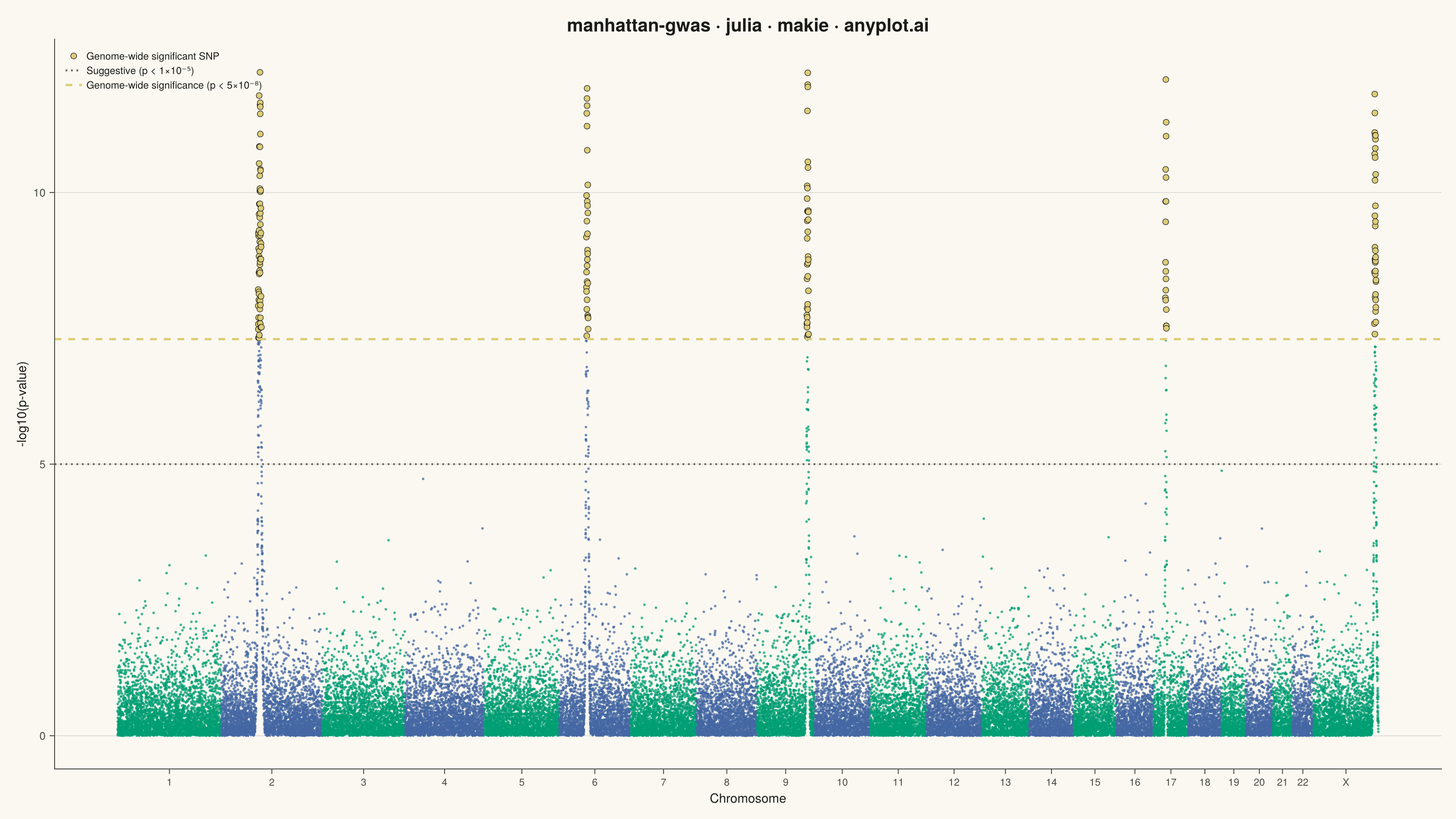
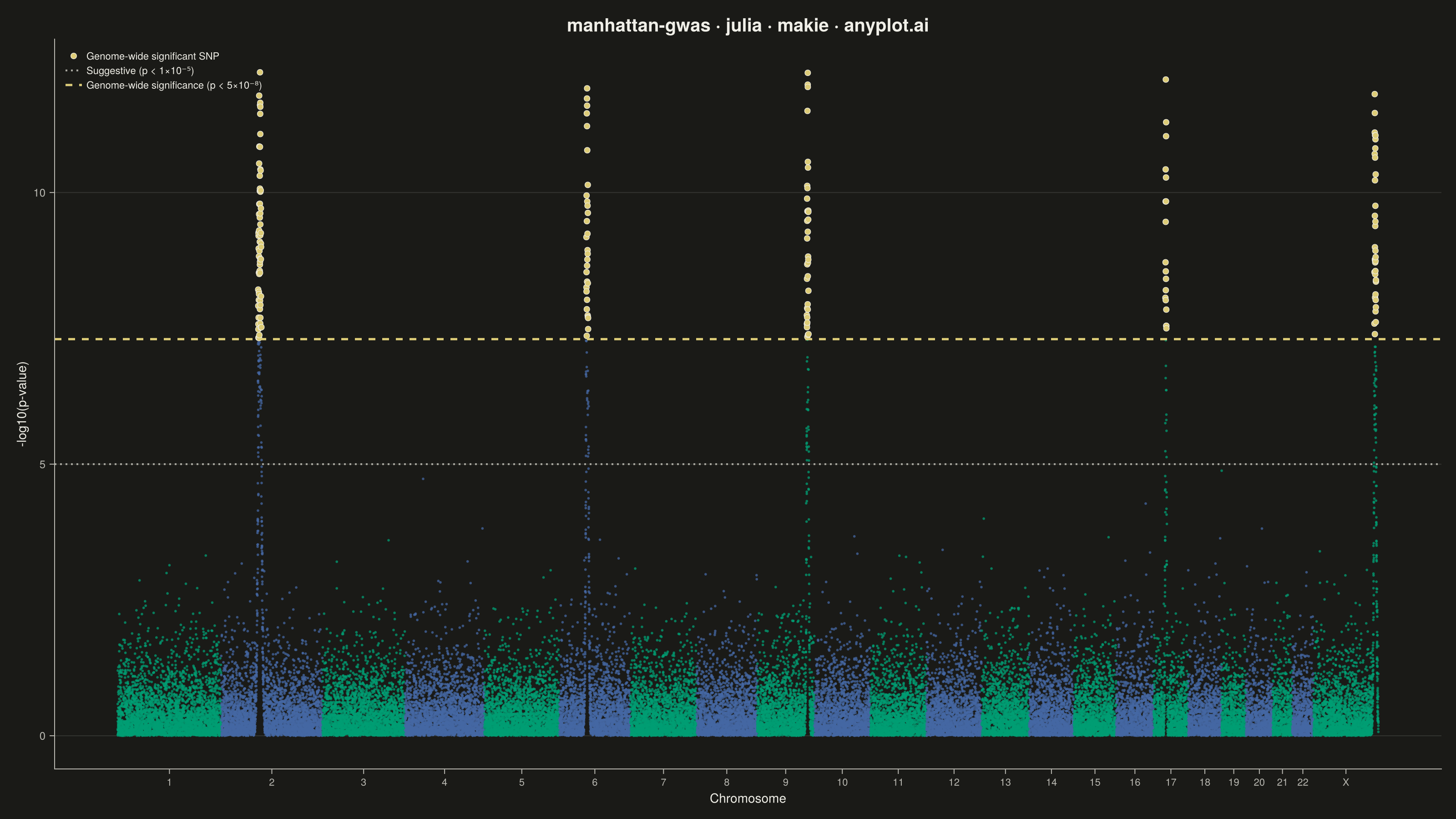
A Manhattan plot visualizes genome-wide association study (GWAS) results by displaying -log10 transformed p-values across chromosomal positions. Points are arranged by genomic position along the x-axis with alternating colors for each chromosome, making it easy to identify significant associations. A horizontal threshold line indicates genome-wide significance (typically p < 5×10⁻⁸). This plot is essential for identifying genetic variants associated with traits or diseases.
# anyplot.ai
# manhattan-gwas: Manhattan Plot for GWAS
# Library: makie 0.21.9 | Julia 1.11.9
# Quality: 88/100 | Created: 2026-09-05

using CairoMakie
using Colors
using Random

Random.seed!(42)

# Theme tokens (see prompts/default-style-guide.md "Theme-adaptive Chrome")
THEME       = get(ENV, "ANYPLOT_THEME", "light")
PAGE_BG     = THEME == "light" ? colorant"#FAF8F1" : colorant"#1A1A17"
ELEVATED_BG = THEME == "light" ? colorant"#FFFDF6" : colorant"#242420"
INK         = THEME == "light" ? colorant"#1A1A17" : colorant"#F0EFE8"
INK_SOFT    = THEME == "light" ? colorant"#4A4A44" : colorant"#B8B7B0"
INK_MUTED   = THEME == "light" ? colorant"#6B6A63" : colorant"#A8A79F"

const IMPRINT_PALETTE = [
    colorant"#009E73", colorant"#C475FD", colorant"#4467A3", colorant"#BD8233",
    colorant"#AE3030", colorant"#2ABCCD", colorant"#954477", colorant"#99B314",
]
CHR_COLOR_ODD  = IMPRINT_PALETTE[1]  # brand green
CHR_COLOR_EVEN = IMPRINT_PALETTE[3]  # blue
AMBER          = colorant"#DDCC77"   # significant-hit highlight

# Data: simulated GWAS summary statistics across the 22 autosomes + chromosome X
chrom_names = vcat(string.(1:22), "X")
chrom_lengths_mb = Float64[
    249, 243, 198, 191, 180, 171, 159, 145, 138, 134, 135, 133,
    114, 107, 102, 90, 83, 80, 59, 64, 47, 51, 156,
]
snps_per_mb = 36.0
peak_chroms = ("2", "6", "9", "17", "X")

chrom_ids  = String[]
positions  = Float64[]
neglog10p  = Float64[]
chrom_centers = Float64[]

top_hit_pos    = Float64[]
top_hit_p      = Float64[]
top_hit_labels = String[]

cumulative_offset = 0.0
for (name, length_mb) in zip(chrom_names, chrom_lengths_mb)
    n_snps = round(Int, length_mb * snps_per_mb)
    local_pos = sort(rand(n_snps) .* length_mb)
    baseline_p = -log10.(rand(n_snps))  # null distribution — mostly non-significant

    if name in peak_chroms
        peak_center = length_mb * rand()
        peak_width = length_mb * 0.015
        peak_signal = 12.0 .* exp.(-((local_pos .- peak_center) .^ 2) ./ (2 * peak_width^2))
        baseline_p = baseline_p .+ peak_signal .* (0.5 .+ 0.5 .* rand(n_snps))

        top_idx = argmax(baseline_p)
        push!(top_hit_pos, local_pos[top_idx] + cumulative_offset)
        push!(top_hit_p, baseline_p[top_idx])
        push!(top_hit_labels, "rs" * string(rand(1_000_000:99_999_999)))
    end

    append!(chrom_ids, fill(name, n_snps))
    append!(positions, local_pos .+ cumulative_offset)
    append!(neglog10p, baseline_p)
    push!(chrom_centers, cumulative_offset + length_mb / 2)

    global cumulative_offset += length_mb
end

point_colors = [isodd(parse_index) ? CHR_COLOR_ODD : CHR_COLOR_EVEN
                for parse_index in indexin(chrom_ids, chrom_names)]

genome_wide_threshold = -log10(5e-8)   # ≈ 7.30 — genome-wide significance
suggestive_threshold  = -log10(1e-5)   # 5.0 — suggestive association

significant = neglog10p .> genome_wide_threshold

# Plot — see default-style-guide.md "Visual Sizing Defaults" for the canvas + sizing values
title_text = "manhattan-gwas · julia · makie · anyplot.ai"

fig = Figure(
    resolution      = (1600, 900),
    fontsize        = 14,
    backgroundcolor = PAGE_BG,
)

ax = Axis(
    fig[1, 1];
    title              = title_text,
    titlesize          = 20,
    titlecolor         = INK,
    xlabel             = "Chromosome",
    ylabel             = "-log10(p-value)",
    xlabelsize         = 14,
    ylabelsize         = 14,
    xlabelcolor        = INK,
    ylabelcolor        = INK,
    xticklabelsize     = 10,
    yticklabelsize     = 12,
    xticklabelcolor    = INK_SOFT,
    yticklabelcolor    = INK_SOFT,
    xtickcolor         = INK_SOFT,
    ytickcolor         = INK_SOFT,
    backgroundcolor    = PAGE_BG,
    topspinevisible    = false,
    rightspinevisible  = false,
    leftspinecolor     = INK_SOFT,
    bottomspinecolor   = INK_SOFT,
    xgridvisible       = false,
    ygridcolor         = RGBAf(INK.r, INK.g, INK.b, 0.12),
    yminorgridvisible  = false,
)
ax.xticks = (chrom_centers, chrom_names)

scatter!(
    ax, positions, neglog10p;
    color = point_colors, markersize = 3, alpha = 0.6, strokewidth = 0,
)
scatter!(
    ax, positions[significant], neglog10p[significant];
    color = AMBER, markersize = 8, strokewidth = 0.6, strokecolor = INK,
    label = "Genome-wide significant SNP",
)

text!(
    ax, top_hit_pos, top_hit_p .+ 0.6;
    text = top_hit_labels, color = INK_SOFT, fontsize = 11,
    align = (:center, :bottom),
)

# Extra headroom above the tallest peak/label keeps the top-left legend box
# (pixel-anchored) clear of the chromosome-2 peak, which otherwise sits
# closest to the axis top among the labeled hits.
ylims!(ax, -0.3, maximum(neglog10p) + 2.5)

hlines!(
    ax, [suggestive_threshold];
    color = INK_MUTED, linestyle = :dot, linewidth = 2,
    label = "Suggestive (p < 1×10⁻⁵)",
)
hlines!(
    ax, [genome_wide_threshold];
    color = AMBER, linestyle = :dash, linewidth = 2.5,
    label = "Genome-wide significance (p < 5×10⁻⁸)",
)

axislegend(
    ax; position = :lt, backgroundcolor = ELEVATED_BG, framevisible = false,
    labelcolor = INK, labelsize = 11, patchsize = (18, 4),
)

# Save
save("plot-$(THEME).png", fig; px_per_unit = 2)
Runnable source as JSON, for any HTTP client: https://api.anyplot.ai/specs/manhattan-gwas/makie/code. Any spec id and library id listed in llms-full.txt fit the same URL shape; every URL below is complete and callable.
{
  "spec_id": "manhattan-gwas",
  "language": "julia",
  "library": "makie",
  "page": "https://anyplot.ai/manhattan-gwas/julia/makie",
  "hub": "https://anyplot.ai/manhattan-gwas",
  "code_json": "https://api.anyplot.ai/specs/manhattan-gwas/makie/code",
  "spec_json": "https://api.anyplot.ai/specs/manhattan-gwas",
  "render_light_png": "https://storage.googleapis.com/anyplot-images/plots/manhattan-gwas/julia/makie/plot-light.png",
  "render_dark_png": "https://storage.googleapis.com/anyplot-images/plots/manhattan-gwas/julia/makie/plot-dark.png",
  "quality_score": 88.0,
  "license": "MIT",
  "guide": "https://anyplot.ai/llms.txt"
}
Part of Manhattan Plot for GWAS on anyplot.ai.