The same plot in 14 other libraries — Python: Altair, Bokeh, lets-plot, Matplotlib, Plotly, plotnine, Pygal, Seaborn; R: ggplot2; JavaScript: Chart.js, D3.js, Apache ECharts, Highcharts, MUI X Charts. Compare all 15 side by side: World Map with Different Projections in Python, R, Julia and JavaScript.
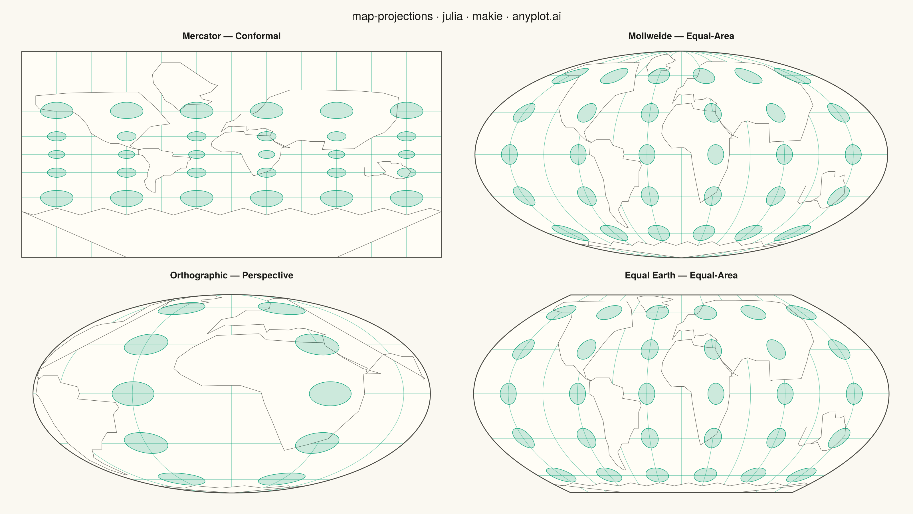
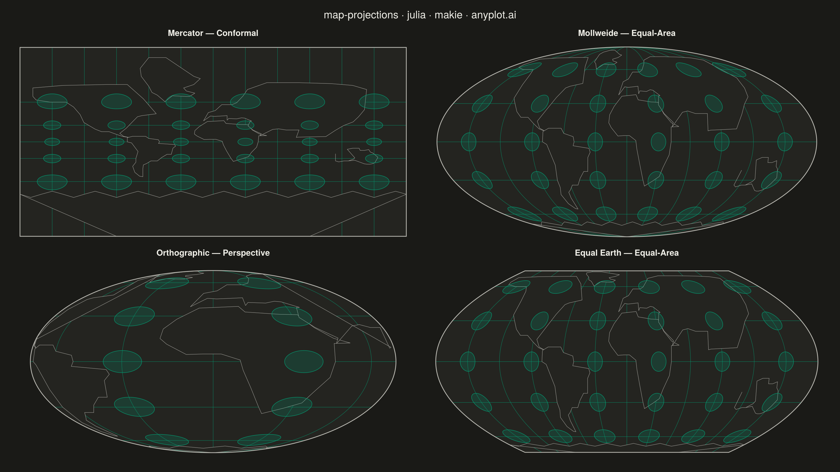
A world map demonstrating different cartographic projections and their distortion characteristics. This visualization showcases how the same geographic data appears under various map projections (Mercator, Robinson, Mollweide, Orthographic, etc.), revealing how each projection preserves or distorts area, shape, distance, or direction. The plot includes graticule (latitude/longitude grid lines) and optionally Tissot indicatrices to illustrate projection distortion patterns.
# anyplot.ai
# map-projections: World Map with Different Projections
# Library: makie 0.22.10 | Julia 1.11.9
# Quality: 86/100 | Created: 2026-05-23

using CairoMakie
using Colors
using Random

Random.seed!(42)

const THEME       = get(ENV, "ANYPLOT_THEME", "light")
const PAGE_BG     = THEME == "light" ? colorant"#FAF8F1" : colorant"#1A1A17"
const ELEVATED_BG = THEME == "light" ? colorant"#FFFDF6" : colorant"#242420"
const INK         = THEME == "light" ? colorant"#1A1A17" : colorant"#F0EFE8"
const INK_SOFT    = THEME == "light" ? colorant"#4A4A44" : colorant"#B8B7B0"
const BRAND       = colorant"#009E73"

d2r(x) = x * π / 180.0

# --- Projection functions ---

function proj_mercator(lon_deg, lat_deg)
    lat = clamp(lat_deg, -85.0, 85.0)
    return d2r(lon_deg), log(tan(π / 4 + d2r(lat) / 2))
end

function mollweide_theta(lat_deg)
    abs(lat_deg) >= 89.9 && return sign(lat_deg) * (π / 2)
    phi   = d2r(lat_deg)
    theta = phi
    rhs   = π * sin(phi)
    for _ in 1:60
        denom = 2.0 + 2.0 * cos(2theta)
        abs(denom) < 1e-14 && break
        theta -= (2theta + sin(2theta) - rhs) / denom
    end
    return theta
end

function proj_mollweide(lon_deg, lat_deg)
    theta = mollweide_theta(lat_deg)
    return (2sqrt(2) / π) * d2r(lon_deg) * cos(theta), sqrt(2) * sin(theta)
end

function proj_orthographic(lon_deg, lat_deg)
    lam = d2r(lon_deg)
    phi = d2r(lat_deg)
    cos(phi) * cos(lam) < 0.0 && return (NaN, NaN)
    return cos(phi) * sin(lam), sin(phi)
end

const EE_M  = sqrt(3.0) / 2.0
const EE_A1 = 1.340264
const EE_A2 = -0.081106
const EE_A3 = 0.000893
const EE_A4 = 0.003796

function proj_equal_earth(lon_deg, lat_deg)
    lam    = d2r(lon_deg)
    phi    = d2r(lat_deg)
    theta  = asin(clamp(EE_M * sin(phi), -1.0, 1.0))
    theta2 = theta * theta
    P      = EE_A1 + theta2 * (EE_A2 + theta2 * (EE_A3 + theta2 * EE_A4))
    return lam * cos(theta) / (EE_M * P), theta * P
end

# --- Simplified continent outlines (lon, lat) in degrees, roughly clockwise ---

const CONTINENT_POLYS = [
    # Africa
    [(-5.4,36.0),(10.0,37.3),(12.0,33.0),(25.0,31.3),(32.5,31.0),
     (36.5,22.0),(43.0,14.8),(50.0,11.8),(42.5,11.5),(42.0,0.0),
     (40.5,-10.0),(35.5,-20.0),(33.0,-27.0),(26.5,-30.8),(18.8,-34.8),
     (16.5,-29.5),(12.5,-17.0),(9.5,-5.5),(8.5,1.0),(2.5,4.8),
     (-3.0,4.8),(-8.5,4.5),(-15.0,11.0),(-17.5,14.7),(-17.0,21.0),
     (-13.0,27.7),(-5.4,36.0)],
    # Eurasia (simplified — Malay Peninsula omitted for clean outline)
    [(-9.0,37.0),(-4.5,48.5),(2.0,51.0),(8.0,57.5),(17.5,57.5),
     (22.0,59.5),(28.0,65.5),(32.0,70.0),(50.0,74.0),(80.0,74.0),
     (110.0,73.5),(130.0,72.5),(143.0,70.0),(141.0,52.0),(135.5,43.0),
     (130.5,35.5),(121.5,29.5),(114.0,21.5),(105.0,10.0),(80.0,9.0),
     (77.5,8.5),(80.0,22.0),(68.0,22.0),(61.0,24.0),(55.5,23.0),
     (44.0,12.0),(43.5,11.5),(45.0,15.0),(37.0,22.0),(32.5,29.0),
     (34.5,36.5),(36.0,36.5),(29.5,41.0),(26.5,41.5),(22.0,40.0),
     (14.5,40.5),(13.0,38.0),(13.0,44.5),(7.5,44.0),(1.5,43.5),
     (-2.5,44.0),(-9.0,37.0)],
    # North America
    [(-168.0,71.0),(-140.0,72.5),(-100.0,73.0),(-80.0,73.0),
     (-65.0,63.0),(-53.0,47.0),(-66.5,44.5),(-70.5,43.0),
     (-75.5,35.0),(-81.0,25.0),(-87.0,16.0),(-83.5,10.5),
     (-77.5,8.0),(-84.0,10.0),(-90.0,14.0),(-97.0,19.0),
     (-104.0,19.0),(-110.0,23.5),(-118.0,32.0),(-120.5,34.5),
     (-124.0,46.0),(-130.0,55.0),(-137.0,60.0),(-152.0,60.0),
     (-165.0,62.0),(-168.0,65.0),(-168.0,71.0)],
    # South America
    [(-80.0,8.0),(-75.0,10.5),(-63.0,10.5),(-60.0,6.5),
     (-51.0,4.0),(-50.0,0.0),(-51.0,-3.0),(-36.0,-5.0),
     (-35.0,-8.0),(-37.5,-12.0),(-39.0,-23.0),(-43.0,-23.0),
     (-48.0,-28.5),(-52.0,-34.0),(-58.0,-34.0),(-62.0,-38.0),
     (-65.0,-40.0),(-65.5,-45.0),(-65.5,-55.0),(-68.5,-54.5),
     (-73.0,-50.0),(-75.0,-42.0),(-72.0,-36.0),(-72.0,-30.0),
     (-70.0,-18.0),(-76.0,-2.0),(-80.0,0.0),(-80.0,8.0)],
    # Australia
    [(114.0,-22.0),(114.0,-34.0),(117.0,-35.5),(122.0,-34.0),
     (126.0,-34.0),(131.0,-31.0),(132.0,-29.0),(125.0,-14.0),
     (130.0,-12.0),(136.0,-12.0),(137.0,-16.0),(141.0,-16.0),
     (145.0,-14.5),(146.5,-19.0),(149.0,-21.0),(153.5,-28.0),
     (152.0,-33.0),(150.5,-37.0),(148.0,-38.5),(146.0,-39.0),
     (143.5,-39.0),(141.0,-38.5),(132.0,-33.0),(126.0,-34.0),
     (122.0,-34.0),(117.0,-35.5),(114.0,-34.0),(114.0,-22.0)],
    # Antarctica — coastal ring then south-pole closure
    [(-180.0,-70.0),(-170.0,-72.0),(-160.0,-70.0),(-150.0,-68.0),
     (-140.0,-70.0),(-130.0,-72.0),(-120.0,-70.0),(-110.0,-68.0),
     (-100.0,-70.0),(-90.0,-72.0),(-80.0,-70.0),(-70.0,-68.0),
     (-60.0,-70.0),(-50.0,-72.0),(-40.0,-70.0),(-30.0,-68.0),
     (-20.0,-70.0),(-10.0,-72.0),(0.0,-70.0),(10.0,-68.0),
     (20.0,-70.0),(30.0,-72.0),(40.0,-70.0),(50.0,-68.0),
     (60.0,-70.0),(70.0,-72.0),(80.0,-70.0),(90.0,-68.0),
     (100.0,-70.0),(110.0,-72.0),(120.0,-70.0),(130.0,-68.0),
     (140.0,-70.0),(150.0,-72.0),(160.0,-70.0),(170.0,-68.0),
     (180.0,-70.0),(90.0,-89.9),(0.0,-89.9),(-90.0,-89.9),
     (-180.0,-70.0)],
    # Greenland (illustrates Mercator distortion)
    [(-44.0,83.0),(-18.0,77.0),(-12.0,76.0),(-18.0,73.0),
     (-27.5,71.0),(-25.0,69.0),(-17.0,67.5),(-22.0,65.0),
     (-25.0,65.0),(-38.0,65.5),(-45.0,60.5),(-52.0,66.0),
     (-57.0,68.0),(-60.0,72.0),(-67.0,77.0),(-68.0,80.0),
     (-60.0,83.0),(-44.0,83.0)],
]

# --- Drawing helpers ---

function draw_lines_nan!(ax, xs, ys; color, linewidth)
    n = length(xs)
    i = 1
    while i <= n
        if !isnan(xs[i]) && !isnan(ys[i])
            j = i + 1
            while j <= n && !isnan(xs[j]) && !isnan(ys[j])
                j += 1
            end
            j > i + 1 && lines!(ax, xs[i:j-1], ys[i:j-1]; color=color, linewidth=linewidth)
            i = j
        else
            i += 1
        end
    end
end

function draw_continents!(ax, proj_fn; fill_color, stroke_color)
    for poly_ll in CONTINENT_POLYS
        pts = Point2f[]
        for (lon, lat) in poly_ll
            x, y = proj_fn(lon, lat)
            !isnan(x) && !isnan(y) && push!(pts, Point2f(x, y))
        end
        length(pts) >= 3 && poly!(ax, pts;
            color=fill_color,
            strokecolor=stroke_color,
            strokewidth=0.7)
    end
end

function draw_graticule!(ax, proj_fn; lon_step=30, lat_step=30, n_pts=200,
                         color=BRAND, linewidth=0.7)
    for lon in -180:lon_step:180
        lats = range(-89.9, 89.9; length=n_pts)
        xs = Float64[]; ys = Float64[]
        for lat in lats
            x, y = proj_fn(lon, lat)
            push!(xs, x); push!(ys, y)
        end
        draw_lines_nan!(ax, xs, ys; color=color, linewidth=linewidth)
    end
    for lat in -90:lat_step:90
        lons = range(-180, 180; length=n_pts)
        xs = Float64[]; ys = Float64[]
        for lon in lons
            x, y = proj_fn(lon, lat)
            push!(xs, x); push!(ys, y)
        end
        draw_lines_nan!(ax, xs, ys; color=color, linewidth=linewidth)
    end
end

function draw_tissot!(ax, proj_fn; fill_color=BRAND, r_deg=7.0, n_pts=60)
    for lon in -150:60:150, lat in -60:30:60
        cos_lat = max(cosd(lat), 0.01)
        pts     = Point2f[]
        any_nan = false
        for k in 0:n_pts-1
            ang    = 2π * k / n_pts
            x, y   = proj_fn(lon + r_deg * sin(ang) / cos_lat,
                             clamp(lat + r_deg * cos(ang), -89.0, 89.0))
            if isnan(x) || isnan(y)
                any_nan = true
            else
                push!(pts, Point2f(x, y))
            end
        end
        !any_nan && length(pts) >= 3 && poly!(ax, pts;
            color=(fill_color, 0.20f0),
            strokecolor=(fill_color, 0.85f0),
            strokewidth=0.9)
    end
end

# --- Projection boundary shapes ---

function boundary_rect(x0, x1, y0, y1)
    [Point2f(x0, y0), Point2f(x1, y0), Point2f(x1, y1), Point2f(x0, y1)]
end

function boundary_ellipse(a, b; n=300)
    ts = range(0, 2π; length=n)
    [Point2f(a * cos(t), b * sin(t)) for t in ts]
end

function boundary_equal_earth(; n=200)
    lats      = collect(range(-90, 90; length=n))
    right     = [Point2f(proj_equal_earth(180, lat)...)  for lat in lats]
    top_pole  = [Point2f(proj_equal_earth(lon, 90)...)   for lon in range(180, -180; length=60)]
    left      = [Point2f(proj_equal_earth(-180, lat)...) for lat in reverse(lats)]
    bot_pole  = [Point2f(proj_equal_earth(lon, -90)...)  for lon in range(-180, 180; length=60)]
    vcat(right, top_pole, left, bot_pole)
end

# --- Layout ---

const merc_y85   = proj_mercator(0, 85.0)[2]
const grat_alpha = THEME == "light" ? 0.55f0 : 0.70f0
const grat_color = RGBAf(Float32(BRAND.r), Float32(BRAND.g), Float32(BRAND.b), grat_alpha)
const bord_color = RGBAf(Float32(INK_SOFT.r), Float32(INK_SOFT.g), Float32(INK_SOFT.b), 1.0f0)
const land_stroke = RGBAf(Float32(INK_SOFT.r), Float32(INK_SOFT.g), Float32(INK_SOFT.b), 0.8f0)

fig = Figure(size=(1600, 900), fontsize=14, backgroundcolor=PAGE_BG)

Label(fig[0, 1:2];
    text="map-projections · julia · makie · anyplot.ai",
    fontsize=20, color=INK, tellwidth=false, padding=(0, 0, 6, 0))

specs = [
    (proj_mercator,     "Mercator — Conformal",       1, 1,
     boundary_rect(-π, π, -merc_y85, merc_y85),
     (-π * 1.06, π * 1.06, -merc_y85 * 1.08, merc_y85 * 1.08)),
    (proj_mollweide,    "Mollweide — Equal-Area",      1, 2,
     boundary_ellipse(2sqrt(2), sqrt(2)),
     (-3.05, 3.05, -1.52, 1.52)),
    (proj_orthographic, "Orthographic — Perspective",  2, 1,
     boundary_ellipse(1.0, 1.0),
     (-1.12, 1.12, -1.12, 1.12)),
    (proj_equal_earth,  "Equal Earth — Equal-Area",    2, 2,
     boundary_equal_earth(),
     (-2.9, 2.9, -1.48, 1.48)),
]

for (proj_fn, title, row, col, bnd_pts, (xlo, xhi, ylo, yhi)) in specs
    ax = Axis(fig[row, col];
        title              = title,
        titlesize          = 16,
        titlecolor         = INK,
        backgroundcolor    = PAGE_BG,
        topspinevisible    = false,
        rightspinevisible  = false,
        leftspinevisible   = false,
        bottomspinevisible = false,
        xticksvisible      = false,
        yticksvisible      = false,
        xticklabelsvisible = false,
        yticklabelsvisible = false,
        xgridvisible       = false,
        ygridvisible       = false,
    )
    xlims!(ax, xlo, xhi)
    ylims!(ax, ylo, yhi)
    poly!(ax, bnd_pts; color=ELEVATED_BG, strokewidth=0)
    draw_graticule!(ax, proj_fn; color=grat_color, linewidth=0.7)
    draw_continents!(ax, proj_fn; fill_color=ELEVATED_BG, stroke_color=land_stroke)
    draw_tissot!(ax, proj_fn; fill_color=BRAND)
    poly!(ax, bnd_pts; color=(:white, 0.0f0), strokecolor=bord_color, strokewidth=1.5)
end

rowgap!(fig.layout, 8)
colgap!(fig.layout, 8)

save("plot-$(THEME).png", fig; px_per_unit=2)
Runnable source as JSON, for any HTTP client: https://api.anyplot.ai/specs/map-projections/makie/code. Any spec id and library id listed in llms-full.txt fit the same URL shape; every URL below is complete and callable.
{
  "spec_id": "map-projections",
  "language": "julia",
  "library": "makie",
  "page": "https://anyplot.ai/map-projections/julia/makie",
  "hub": "https://anyplot.ai/map-projections",
  "code_json": "https://api.anyplot.ai/specs/map-projections/makie/code",
  "spec_json": "https://api.anyplot.ai/specs/map-projections",
  "render_light_png": "https://storage.googleapis.com/anyplot-images/plots/map-projections/julia/makie/plot-light.png",
  "render_dark_png": "https://storage.googleapis.com/anyplot-images/plots/map-projections/julia/makie/plot-dark.png",
  "quality_score": 86.0,
  "license": "MIT",
  "guide": "https://anyplot.ai/llms.txt"
}
Part of World Map with Different Projections on anyplot.ai.