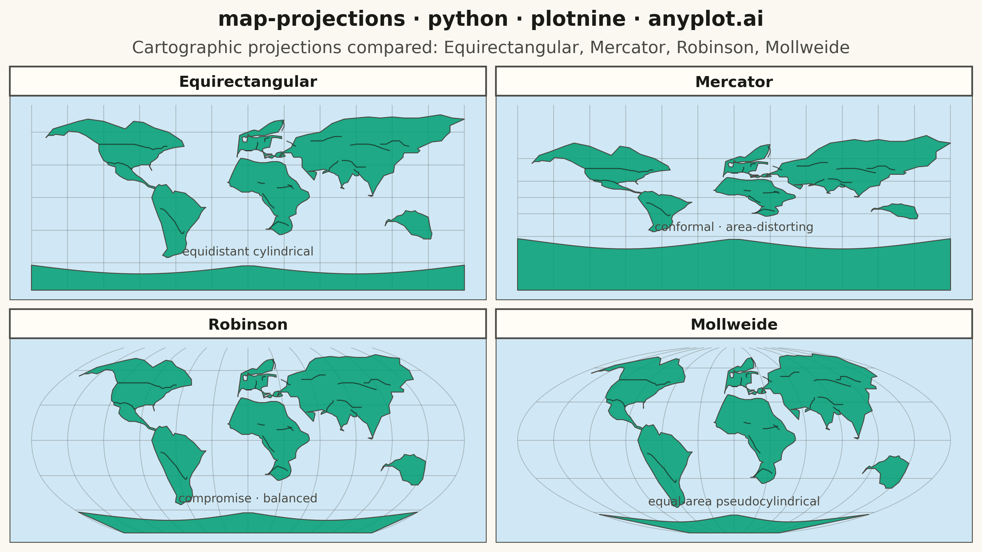
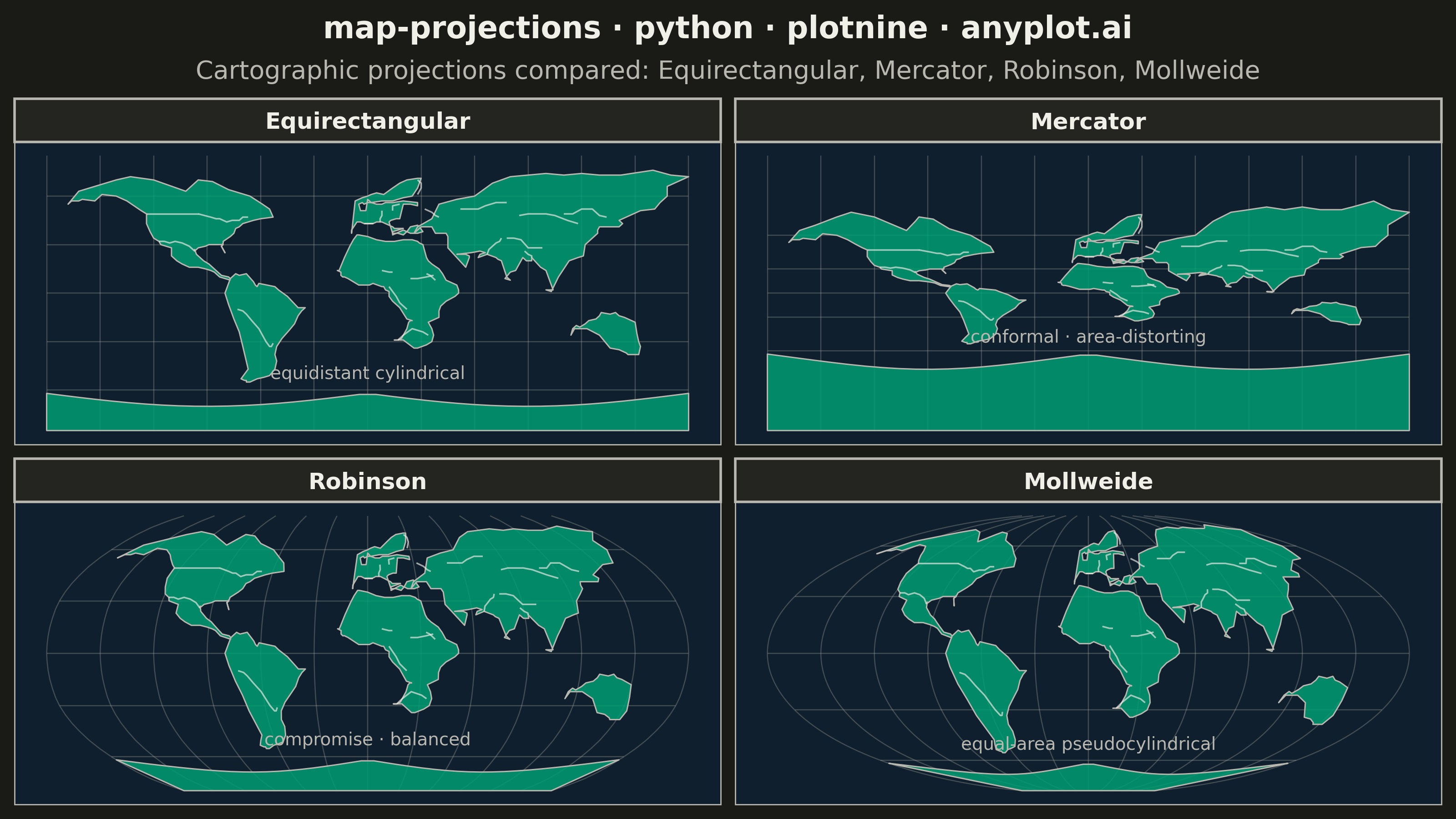
A world map demonstrating different cartographic projections and their distortion characteristics. This visualization showcases how the same geographic data appears under various map projections (Mercator, Robinson, Mollweide, Orthographic, etc.), revealing how each projection preserves or distorts area, shape, distance, or direction. The plot includes graticule (latitude/longitude grid lines) and optionally Tissot indicatrices to illustrate projection distortion patterns.
""" anyplot.ai
map-projections: World Map with Different Projections
Library: plotnine 0.15.4 | Python 3.13.13
Quality: 89/100 | Updated: 2026-05-23
"""
import os
import sys
# Remove the script's own directory from sys.path so 'plotnine' resolves to
# the installed package, not this file (which shares the same name).
_here = os.path.dirname(os.path.abspath(__file__))
sys.path = [p for p in sys.path if os.path.abspath(p) != _here]
import numpy as np
import pandas as pd
from plotnine import (
aes,
coord_fixed,
element_blank,
element_rect,
element_text,
facet_wrap,
geom_path,
geom_polygon,
geom_text,
ggplot,
labs,
theme,
)
THEME = os.getenv("ANYPLOT_THEME", "light")
PAGE_BG = "#FAF8F1" if THEME == "light" else "#1A1A17"
ELEVATED_BG = "#FFFDF6" if THEME == "light" else "#242420"
INK = "#1A1A17" if THEME == "light" else "#F0EFE8"
INK_SOFT = "#4A4A44" if THEME == "light" else "#B8B7B0"
LAND_COLOR = "#009E73"
OCEAN_BG = "#D0E8F5" if THEME == "light" else "#0F1F2D"
np.random.seed(42)
# Robinson projection lookup table
_LAT = np.array([0, 5, 10, 15, 20, 25, 30, 35, 40, 45, 50, 55, 60, 65, 70, 75, 80, 85, 90])
_XF = np.array(
[
1.0,
0.9986,
0.9954,
0.99,
0.9822,
0.973,
0.96,
0.9427,
0.9216,
0.8962,
0.8679,
0.835,
0.7986,
0.7597,
0.7186,
0.6732,
0.6213,
0.5722,
0.5322,
]
)
_YF = np.array(
[
0.0,
0.062,
0.124,
0.186,
0.248,
0.31,
0.372,
0.434,
0.4958,
0.5571,
0.6176,
0.6769,
0.7346,
0.7903,
0.8435,
0.8936,
0.9394,
0.9761,
1.0,
]
)
def _mollweide(lon, lat):
la = np.radians(lat)
t = la.copy()
for _ in range(15):
den = 2 + 2 * np.cos(2 * t)
den = np.where(np.abs(den) < 1e-10, 1e-10, den)
t -= (2 * t + np.sin(2 * t) - np.pi * np.sin(la)) / den
return 2 * np.sqrt(2) / np.pi * np.radians(lon) * np.cos(t), np.sqrt(2) * np.sin(t)
PROJ_FNS = {
"Equirectangular": lambda lon, lat: (np.radians(lon), np.radians(lat)),
"Mercator": lambda lon, lat: (np.radians(lon), np.log(np.tan(np.pi / 4 + np.radians(np.clip(lat, -85, 85)) / 2))),
"Robinson": lambda lon, lat: (
np.radians(lon) * np.interp(np.abs(lat), _LAT, _XF) * 0.8487,
np.interp(np.abs(lat), _LAT, _YF) * np.sign(lat) * 1.3523,
),
"Mollweide": _mollweide,
}
# === Continent coastlines ===
# Coordinates trace outer boundary; enough points to be recognizable at map scale
# North America: Alaska -> Pacific coast -> Mexico/Central Am -> Gulf -> Florida ->
# East coast -> Maritime Canada -> Northern Canada -> back
_NA_LON = np.array(
[
-168,
-166,
-162,
-160,
-153,
-149,
-141, # Alaska W peninsula -> SE Alaska
-135,
-131,
-127,
-124, # BC coast to US border
-124,
-124,
-122,
-120,
-117, # WA/OR/CA
-116,
-110,
-110,
-107,
-104,
-100,
-95, # Baja/Mexico Pacific/Tehuantepec
-91,
-88,
-86,
-83,
-80,
-77, # Central America (Pacific side)
-77,
-78,
-82,
-85,
-87,
-89,
-92,
-96,
-97, # Panama->Gulf coast W
-97,
-95,
-91,
-89,
-86,
-84,
-81, # TX/LA/MS/AL/FL panhandle
-82,
-80,
-80,
-82,
-81, # Florida
-81,
-77,
-75,
-74,
-72,
-71,
-70,
-67,
-64, # East coast
-60,
-53,
-55,
-59, # Maritime/Newfoundland
-66,
-78,
-87,
-95,
-97, # Hudson Strait / NW Hudson Bay
-102,
-120,
-133,
-141,
-153,
-162,
-168, # N Canada / Arctic coast
]
)
_NA_LAT = np.array(
[
55,
57,
57,
58,
57,
61,
60,
57,
54,
51,
49,
47,
43,
38,
34,
32,
30,
28,
23,
20,
18,
16,
16,
15,
14,
13,
10,
9,
8,
9,
10,
11,
14,
16,
18,
20,
24,
27,
26,
28,
29,
30,
30,
30,
30,
29,
25,
25,
29,
31,
32,
35,
37,
40,
41,
42,
43,
44,
45,
46,
47,
52,
55,
60,
64,
69,
70,
68,
63,
70,
72,
70,
66,
63,
55,
]
)
# South America: Caribbean coast -> NE Brazil -> SE/S Brazil -> Patagonia ->
# Cape Horn -> Chile Pacific -> Colombia Pacific -> back
_SA_LON = np.array(
[
-77,
-74,
-72,
-68,
-64,
-63,
-62,
-61, # Caribbean (Panama->Trinidad area)
-52,
-50,
-45,
-39,
-35, # NE Brazil coast
-37,
-39,
-41,
-44,
-48,
-51, # SE Brazil
-52,
-51,
-52,
-55,
-58,
-62,
-66,
-68, # S Argentina / Patagonia
-68,
-69,
-71,
-69,
-67, # Tierra del Fuego / Cape Horn
-70,
-72,
-75,
-78,
-80, # Chile Pacific coast north
-77, # Colombia Pacific / back to start
]
)
_SA_LAT = np.array(
[
9,
12,
11,
12,
7,
5,
4,
6,
4,
2,
-2,
-9,
-9,
-11,
-14,
-19,
-23,
-28,
-33,
-38,
-42,
-47,
-51,
-52,
-53,
-55,
-55,
-54,
-54,
-53,
-50,
-47,
-33,
-24,
-16,
-7,
0,
9,
]
)
# Europe: Iberia -> Bay of Biscay -> France -> N Sea -> Scandinavia ->
# Baltic -> E Europe -> Balkans -> Adriatic -> Apennines -> Iberia
_EU_LON = np.array(
[
-9,
-9,
-6,
-4,
-2,
0,
2,
3, # Portugal/Spain south -> Gibraltar -> France
5,
7,
8,
10,
14,
15,
18,
20, # Riviera -> Italy W coast -> Adriatic
14,
14,
16,
20,
24,
26,
28,
31, # Italy toe -> Adriatic -> Greece -> Turkey W
29,
28,
24,
22,
20,
17,
14, # Black Sea coast -> Greece back
12,
13,
16,
18,
20,
24,
28,
28, # Adriatic E -> Balkans -> Poland
20,
14,
10,
8,
5,
2,
0, # Poland -> Germany -> North Sea
-1,
-4,
-5,
-3,
-2,
0, # Netherlands/Belgium -> S England (omit island)
2,
8,
14,
20,
25,
28, # Denmark / Sweden / Finland
30,
28,
22,
18,
14,
9, # Baltic north / Norway -> Scandinavia
5,
2,
0,
-3,
-7,
-9, # Norway W coast / Scotland area -> Portugal
-9,
]
)
_EU_LAT = np.array(
[
37,
39,
44,
44,
43,
43,
43,
43,
44,
44,
44,
43,
41,
40,
40,
40,
38,
36,
37,
39,
37,
37,
37,
38,
41,
42,
41,
38,
36,
37,
37,
44,
45,
46,
46,
55,
55,
54,
56,
57,
56,
56,
55,
55,
56,
58,
51,
51,
55,
56,
55,
56,
56,
57,
57,
59,
60,
65,
71,
71,
70,
68,
65,
61,
62,
61,
60,
59,
57,
37,
37,
]
)
# Africa: Morocco -> NW coast -> Gulf of Guinea -> Congo -> S Africa ->
# E Africa -> Horn -> Red Sea / Suez -> N Africa -> Morocco
_AF_LON = np.array(
[
-5,
-6,
-8,
-10,
-13,
-16,
-17, # Morocco -> Dakar (Senegal)
-15,
-15,
-14,
-13,
-11,
-8, # Guinea coast
-5,
-2,
1,
3,
8,
9, # Ghana -> Nigeria -> Cameroon
9,
10,
12,
12,
14,
18,
22,
25, # Cameroon -> Gabon -> Congo -> Angola
24,
23,
22,
19,
17, # Angola south
15,
17,
20,
26,
28,
33,
36, # Namibia -> S Africa -> Cape -> E Cape
37,
36,
34,
40,
40,
41,
44, # Mozambique -> Tanzania -> Kenya -> Somalia
49,
51,
51,
50,
44,
43,
42, # Somalia (Horn)
40,
36,
34,
33,
31,
29,
28, # Red Sea W -> Sudan/Eritrea -> Egypt
25,
20,
15,
10,
5,
0,
-5, # Libya -> Tunisia -> Algeria -> Morocco
-5,
]
)
_AF_LAT = np.array(
[
36,
36,
33,
29,
22,
14,
14,
13,
11,
10,
10,
9,
7,
5,
5,
5,
6,
4,
4,
4,
2,
1,
-2,
-5,
-9,
-16,
-17,
-17,
-18,
-22,
-28,
-29,
-29,
-29,
-29,
-34,
-34,
-32,
-30,
-26,
-22,
-18,
-15,
-11,
-8,
-5,
-2,
0,
2,
5,
8,
10,
12,
15,
18,
20,
22,
30,
31,
32,
33,
33,
32,
32,
33,
35,
36,
36,
]
)
# Asia: Turkey -> Middle East -> Arabian Peninsula -> India -> SE Asia ->
# China coast -> Korea/Japan coast -> Russia Far East -> Siberia/Arctic -> Turkey
_AS_LON = np.array(
[
26,
30,
36,
38,
41,
44,
45, # Turkey -> Syria -> Red Sea -> Yemen W
45,
50,
55,
57,
57,
55,
50, # Yemen -> Oman -> Gulf of Oman
58,
63,
66,
63,
62, # Pakistan coast
67,
72,
73,
75,
78,
80,
80, # India W coast -> Gujarat -> tip
77,
80,
83,
87,
89,
92, # India E coast
92,
97,
100,
104,
103,
100, # Bangladesh -> Myanmar -> Thailand/Malay
103,
107,
110,
113,
118,
121,
122, # Vietnam coast -> China coast
126,
129,
129,
130,
131,
141,
143, # Korea -> Vladivostok -> Sakhalin -> Japan coast
141,
153,
161,
164,
168,
168, # Hokkaido coast -> Kamchatka -> Chukotka
180,
170,
160,
148,
142,
135, # E Siberia / Arctic coast
130,
120,
110,
100,
90,
80,
70, # N Siberia / Russia Arctic coast
60,
50,
40,
36,
28,
26, # Ural -> Caspian -> Caucasus -> Turkey N
26,
]
)
_AS_LAT = np.array(
[
37,
41,
41,
37,
37,
37,
35,
28,
22,
16,
22,
23,
24,
24,
25,
26,
25,
24,
22,
24,
22,
21,
20,
10,
8,
8,
9,
13,
14,
22,
20,
20,
22,
16,
14,
2,
2,
2,
1,
10,
15,
20,
22,
23,
30,
34,
37,
39,
41,
41,
41,
43,
45,
51,
52,
56,
60,
66,
72,
73,
76,
74,
73,
73,
73,
74,
73,
74,
73,
72,
68,
60,
58,
55,
46,
41,
37,
]
)
# Australia
_AU_LON = np.array(
[
114,
115,
117,
119,
122,
124,
128,
130, # SW coast -> S Australia
131,
136,
139,
141,
144,
146, # SA -> Victoria
150,
151,
152,
153,
152,
150, # NSW -> Queensland N coast
148,
146,
145,
141,
136,
130,
123,
116, # Cape York -> N coast -> NW
114,
]
)
_AU_LAT = np.array(
[
-26,
-22,
-20,
-21,
-19,
-17,
-16,
-14,
-12,
-13,
-12,
-14,
-15,
-16,
-18,
-25,
-30,
-33,
-38,
-38,
-38,
-38,
-37,
-35,
-34,
-26,
-22,
-22,
-26,
]
)
# Antarctica (keep as formula-based)
_AN_LON = np.linspace(-180, 180, 40)
_AN_LAT_N = np.array([-62 - 8 * np.abs(np.sin(np.radians(lo))) for lo in _AN_LON])
_AN_LON_F = np.concatenate([_AN_LON, _AN_LON[::-1], [_AN_LON[0]]])
_AN_LAT_F = np.concatenate([_AN_LAT_N, np.full(40, -85), [_AN_LAT_N[0]]])
continents_raw = [
("North America", _NA_LON, _NA_LAT),
("South America", _SA_LON, _SA_LAT),
("Europe", _EU_LON, _EU_LAT),
("Africa", _AF_LON, _AF_LAT),
("Asia", _AS_LON, _AS_LAT),
("Australia", _AU_LON, _AU_LAT),
("Antarctica", _AN_LON_F, _AN_LAT_F),
]
# === Country borders (major borders as path lines) ===
# Each entry: (name, lon_array, lat_array)
# Coordinates approximate key turning points of the border
_borders_raw = [
# USA–Canada: 49th parallel (Pacific -> Great Lakes area -> Maine)
("US-CAN-W", np.array([-124, -120, -115, -110, -105, -100, -95]), np.array([49, 49, 49, 49, 49, 49, 49])),
(
"US-CAN-E",
np.array([-95, -88, -85, -83, -79, -76, -72, -70, -67]),
np.array([49, 47, 46, 46, 44, 45, 45, 47, 47]),
),
# USA–Mexico border (Pacific -> Rio Grande -> Gulf)
("US-MEX", np.array([-117, -114, -111, -108, -104, -100, -97]), np.array([32, 32, 31, 32, 31, 29, 26])),
# Brazil–Bolivia/Peru
("BR-W", np.array([-73, -70, -68, -65, -61, -58]), np.array([-10, -11, -13, -17, -22, -28])),
# Brazil–Argentina/Paraguay
("BR-S", np.array([-58, -57, -55, -54, -53]), np.array([-28, -30, -33, -33, -31])),
# India borders (Pakistan W + Bangladesh E)
("IND-PAK", np.array([67, 68, 70, 72, 74, 75]), np.array([24, 27, 29, 31, 32, 34])),
("IND-BGD", np.array([88, 89, 90, 92, 92]), np.array([26, 25, 24, 23, 22])),
# China–Russia (Amur River)
("CHN-RUS", np.array([110, 115, 120, 126, 130, 134]), np.array([49, 49, 52, 52, 48, 47])),
# China–Mongolia
("CHN-MNG", np.array([85, 90, 95, 100, 105, 112, 118]), np.array([48, 49, 49, 49, 48, 45, 43])),
# China–India (LAC line, simplified)
("CHN-IND", np.array([78, 82, 86, 90, 94, 98]), np.array([34, 34, 33, 28, 28, 28])),
# Russia–Kazakhstan (approximate W segment)
("RUS-KAZ", np.array([52, 58, 62, 66, 72, 78]), np.array([52, 52, 52, 54, 56, 56])),
# European borders (key recognizable ones)
# France–Spain (Pyrenees)
("FR-ES", np.array([-2, 0, 2, 3]), np.array([43, 43, 43, 43])),
# France–Italy / France–Germany (Alps/Rhine)
("FR-IT-DE", np.array([7, 7, 8, 8]), np.array([44, 46, 48, 51])),
# Germany–Poland (Oder-Neisse)
("DE-PL", np.array([14, 14, 18]), np.array([51, 54, 55])),
# Ukraine–Russia (approximate)
("UA-RU", np.array([32, 36, 38, 40]), np.array([52, 50, 48, 47])),
# Finland–Russia
("FI-RU", np.array([28, 29, 30, 30, 28]), np.array([61, 63, 65, 68, 70])),
# Africa: Sudan–South Sudan
("SDN-SSD", np.array([24, 28, 33, 37]), np.array([9, 9, 10, 11])),
# Africa: Congo DRC border (simplified)
("COD-W", np.array([12, 16, 18, 22]), np.array([4, -2, -6, -10])),
# Africa: South Africa borders
("ZAF-N", np.array([17, 20, 25, 28, 31, 34]), np.array([-29, -26, -22, -23, -24, -26])),
# Africa: Nigeria–Chad (Lake Chad area)
("NGA-TCD", np.array([8, 12, 14]), np.array([14, 13, 13])),
# Africa: Ethiopia–Sudan
("ETH-SDN", np.array([33, 35, 38]), np.array([12, 11, 8])),
]
# Build continent DataFrame
cont_records = []
for name, lons, lats in continents_raw:
for i, (lo, la) in enumerate(zip(lons, lats, strict=False)):
cont_records.append({"continent": name, "order": i, "lon": lo, "lat": la})
df_cont = pd.DataFrame(cont_records)
# Build borders DataFrame
bord_records = []
for seg_id, (name, lons, lats) in enumerate(_borders_raw):
for i, (lo, la) in enumerate(zip(lons, lats, strict=False)):
bord_records.append({"border": name, "seg": seg_id, "order": i, "lon": lo, "lat": la})
df_bord = pd.DataFrame(bord_records)
# Build graticule DataFrame
grat_records = []
for lo_val in range(-180, 181, 30):
lats = np.linspace(-85, 85, 200)
for i, la_val in enumerate(lats):
grat_records.append({"group": f"lon_{lo_val}", "lon": lo_val, "lat": la_val, "order": i})
for la_val in range(-60, 61, 30):
lons = np.linspace(-180, 180, 300)
for i, lo_val in enumerate(lons):
grat_records.append({"group": f"lat_{la_val}", "lon": lo_val, "lat": la_val, "order": i})
df_grat = pd.DataFrame(grat_records)
# Apply projections
proj_order = ["Equirectangular", "Mercator", "Robinson", "Mollweide"]
all_cont, all_grat, all_bord = [], [], []
for proj in proj_order:
fn = PROJ_FNS[proj]
pc = df_cont.copy()
pc["x"], pc["y"] = fn(pc["lon"].values, pc["lat"].values)
pc["projection"] = proj
pc["proj_continent"] = proj + "_" + pc["continent"]
all_cont.append(pc)
pg = df_grat.copy()
pg["x"], pg["y"] = fn(pg["lon"].values, pg["lat"].values)
pg["projection"] = proj
pg["proj_group"] = proj + "_" + pg["group"]
all_grat.append(pg)
pb = df_bord.copy()
pb["x"], pb["y"] = fn(pb["lon"].values, pb["lat"].values)
pb["projection"] = proj
pb["proj_border"] = proj + "_" + pb["border"]
all_bord.append(pb)
df_all_cont = pd.concat(all_cont, ignore_index=True)
df_all_grat = pd.concat(all_grat, ignore_index=True)
df_all_bord = pd.concat(all_bord, ignore_index=True)
for df in (df_all_cont, df_all_grat, df_all_bord):
df["projection"] = pd.Categorical(df["projection"], categories=proj_order, ordered=True)
# Per-panel distortion annotations (DE-03)
PROJ_NOTES = {
"Equirectangular": "equidistant cylindrical",
"Mercator": "conformal · area-distorting",
"Robinson": "compromise · balanced",
"Mollweide": "equal-area pseudocylindrical",
}
annot_records = []
for proj in proj_order:
x_a, y_a = PROJ_FNS[proj](np.array([0.0]), np.array([-50.0]))
annot_records.append({"projection": proj, "x": float(x_a[0]), "y": float(y_a[0]), "label": PROJ_NOTES[proj]})
df_annot = pd.DataFrame(annot_records)
df_annot["projection"] = pd.Categorical(df_annot["projection"], categories=proj_order, ordered=True)
# Plot
plot = (
ggplot()
+ geom_path(aes(x="x", y="y", group="proj_group"), data=df_all_grat, color=INK_SOFT, size=0.25, alpha=0.3)
+ geom_polygon(
aes(x="x", y="y", group="proj_continent"),
data=df_all_cont,
fill=LAND_COLOR,
color=INK_SOFT,
size=0.3,
alpha=0.85,
)
+ geom_path(aes(x="x", y="y", group="proj_border"), data=df_all_bord, color=INK, size=0.35, alpha=0.65)
+ geom_text(aes(x="x", y="y", label="label"), data=df_annot, color=INK_SOFT, size=7, ha="center")
+ facet_wrap("~projection", ncol=2, scales="free")
+ coord_fixed(ratio=1.0)
+ labs(
title="map-projections · python · plotnine · anyplot.ai",
subtitle="Cartographic projections compared: Equirectangular, Mercator, Robinson, Mollweide",
)
+ theme(
figure_size=(8, 4.5),
plot_title=element_text(size=12, weight="bold", ha="center", color=INK),
plot_subtitle=element_text(size=10, ha="center", color=INK_SOFT),
strip_text=element_text(size=9, weight="bold", color=INK),
strip_background=element_rect(fill=ELEVATED_BG, color=INK_SOFT),
axis_text=element_blank(),
axis_title=element_blank(),
axis_ticks=element_blank(),
panel_grid=element_blank(),
panel_background=element_rect(fill=OCEAN_BG),
panel_border=element_rect(color=INK_SOFT, fill=None, size=0.5),
plot_background=element_rect(fill=PAGE_BG, color=PAGE_BG),
legend_position="none",
)
)
plot.save(f"plot-{THEME}.png", dpi=400, width=8, height=4.5, units="in")
Runnable source as JSON, for any HTTP client: https://api.anyplot.ai/specs/map-projections/plotnine/code. Any spec id and library id listed in llms-full.txt fit the same URL shape; every URL below is complete and callable.
{
  "spec_id": "map-projections",
  "language": "python",
  "library": "plotnine",
  "page": "https://anyplot.ai/map-projections/python/plotnine",
  "hub": "https://anyplot.ai/map-projections",
  "code_json": "https://api.anyplot.ai/specs/map-projections/plotnine/code",
  "spec_json": "https://api.anyplot.ai/specs/map-projections",
  "render_light_png": "https://storage.googleapis.com/anyplot-images/plots/map-projections/python/plotnine/plot-light.png",
  "render_dark_png": "https://storage.googleapis.com/anyplot-images/plots/map-projections/python/plotnine/plot-dark.png",
  "quality_score": 89.0,
  "license": "MIT",
  "guide": "https://anyplot.ai/llms.txt"
}
Part of World Map with Different Projections on anyplot.ai.