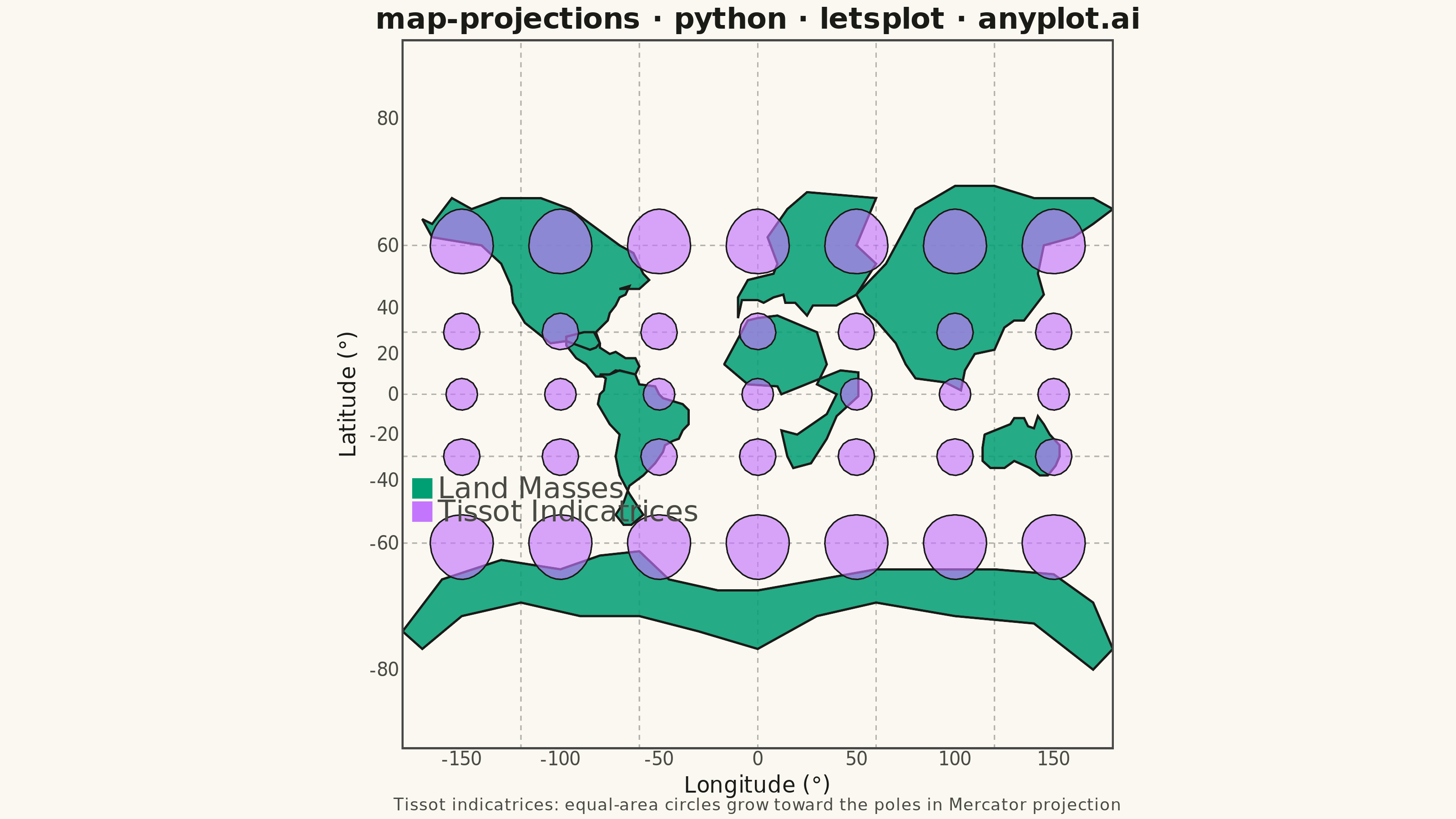
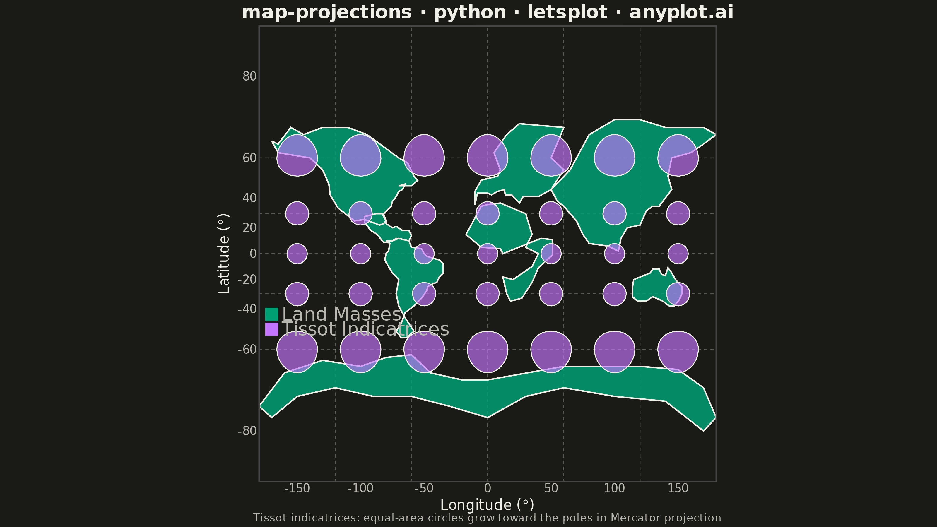
A world map demonstrating different cartographic projections and their distortion characteristics. This visualization showcases how the same geographic data appears under various map projections (Mercator, Robinson, Mollweide, Orthographic, etc.), revealing how each projection preserves or distorts area, shape, distance, or direction. The plot includes graticule (latitude/longitude grid lines) and optionally Tissot indicatrices to illustrate projection distortion patterns.
""" anyplot.ai
map-projections: World Map with Different Projections
Library: letsplot 4.10.1 | Python 3.13.13
Quality: 83/100 | Updated: 2026-05-23
"""

import os

import numpy as np
import pandas as pd
from lets_plot import (
    LetsPlot,
    aes,
    coord_map,
    element_blank,
    element_rect,
    element_text,
    geom_path,
    geom_point,
    geom_polygon,
    geom_text,
    ggplot,
    ggsize,
    labs,
    scale_color_identity,
    theme,
    theme_minimal,
)
from lets_plot.export import ggsave
from PIL import Image as PILImage


LetsPlot.setup_html()

THEME = os.getenv("ANYPLOT_THEME", "light")
PAGE_BG = "#FAF8F1" if THEME == "light" else "#1A1A17"
INK = "#1A1A17" if THEME == "light" else "#F0EFE8"
INK_SOFT = "#4A4A44" if THEME == "light" else "#B8B7B0"

IMPRINT = ["#009E73", "#C475FD", "#AE3030", "#4467A3", "#99B314", "#954477", "#BD8233"]
LAND_COLOR = IMPRINT[0]  # brand green — first categorical series
TISSOT_COLOR = IMPRINT[1]  # purple — canonical second series

np.random.seed(42)

# Data: Generate graticule lines (lat/lon grid)
graticule_rows = []
line_id = 0

for lat in range(-90, 91, 30):
    lons = np.linspace(-180, 180, 180)
    for lon in lons:
        graticule_rows.append({"lon": lon, "lat": lat, "line_id": line_id})
    line_id += 1

for lon in range(-180, 181, 60):
    lats = np.linspace(-90, 90, 180)
    for lat in lats:
        graticule_rows.append({"lon": lon, "lat": lat, "line_id": line_id})
    line_id += 1

graticule = pd.DataFrame(graticule_rows)

# Data: Continent outlines
continent_rows = []

africa_coords = [
    (-17, 15),
    (-5, 5),
    (10, 4),
    (12, 0),
    (42, 12),
    (51, 11),
    (51, -1),
    (40, -11),
    (35, -22),
    (27, -33),
    (18, -35),
    (15, -30),
    (12, -18),
    (20, -20),
    (35, -10),
    (40, 0),
    (30, 5),
    (35, 15),
    (30, 30),
    (10, 37),
    (0, 36),
    (-5, 35),
    (-17, 15),
]
for lon, lat in africa_coords:
    continent_rows.append({"lon": lon, "lat": lat, "continent": "Africa"})

europe_coords = [
    (-10, 36),
    (-8, 43),
    (0, 43),
    (3, 42),
    (8, 44),
    (13, 45),
    (14, 42),
    (19, 42),
    (25, 37),
    (28, 41),
    (40, 41),
    (50, 45),
    (55, 50),
    (60, 55),
    (50, 60),
    (60, 70),
    (25, 71),
    (15, 68),
    (5, 62),
    (10, 55),
    (8, 52),
    (-5, 50),
    (-10, 44),
    (-10, 36),
]
for lon, lat in europe_coords:
    continent_rows.append({"lon": lon, "lat": lat, "continent": "Europe"})

asia_coords = [
    (60, 35),
    (70, 25),
    (75, 15),
    (80, 8),
    (95, 6),
    (103, 2),
    (105, 12),
    (110, 20),
    (120, 22),
    (125, 32),
    (130, 35),
    (135, 35),
    (140, 40),
    (145, 45),
    (142, 52),
    (145, 60),
    (160, 62),
    (170, 65),
    (180, 68),
    (170, 70),
    (140, 70),
    (120, 72),
    (100, 72),
    (80, 68),
    (65, 55),
    (50, 45),
    (55, 38),
    (60, 35),
]
for lon, lat in asia_coords:
    continent_rows.append({"lon": lon, "lat": lat, "continent": "Asia"})

na_coords = [
    (-170, 66),
    (-165, 62),
    (-140, 60),
    (-130, 55),
    (-125, 48),
    (-124, 42),
    (-118, 34),
    (-105, 25),
    (-97, 26),
    (-85, 22),
    (-82, 23),
    (-80, 25),
    (-83, 30),
    (-88, 30),
    (-92, 29),
    (-97, 28),
    (-97, 24),
    (-92, 18),
    (-87, 15),
    (-82, 9),
    (-78, 9),
    (-75, 10),
    (-72, 12),
    (-62, 10),
    (-60, 14),
    (-62, 18),
    (-65, 18),
    (-67, 18),
    (-72, 21),
    (-75, 20),
    (-80, 23),
    (-80, 25),
    (-82, 30),
    (-76, 35),
    (-75, 38),
    (-72, 41),
    (-70, 44),
    (-67, 45),
    (-65, 48),
    (-70, 47),
    (-60, 47),
    (-55, 50),
    (-58, 52),
    (-63, 58),
    (-70, 60),
    (-85, 65),
    (-95, 68),
    (-110, 70),
    (-130, 70),
    (-145, 68),
    (-155, 70),
    (-165, 65),
    (-170, 66),
]
for lon, lat in na_coords:
    continent_rows.append({"lon": lon, "lat": lat, "continent": "North America"})

sa_coords = [
    (-80, 10),
    (-75, 10),
    (-70, 12),
    (-62, 10),
    (-60, 5),
    (-52, 4),
    (-50, 0),
    (-48, -2),
    (-44, -3),
    (-38, -5),
    (-35, -8),
    (-35, -15),
    (-38, -18),
    (-40, -22),
    (-43, -23),
    (-47, -25),
    (-48, -28),
    (-52, -33),
    (-58, -38),
    (-65, -42),
    (-68, -48),
    (-72, -52),
    (-68, -55),
    (-64, -55),
    (-58, -52),
    (-65, -45),
    (-70, -38),
    (-72, -30),
    (-70, -20),
    (-75, -15),
    (-81, -5),
    (-80, 0),
    (-78, 2),
    (-77, 8),
    (-80, 10),
]
for lon, lat in sa_coords:
    continent_rows.append({"lon": lon, "lat": lat, "continent": "South America"})

aus_coords = [
    (115, -20),
    (120, -18),
    (128, -15),
    (130, -12),
    (135, -12),
    (137, -16),
    (140, -17),
    (142, -11),
    (145, -15),
    (148, -20),
    (153, -25),
    (153, -30),
    (151, -34),
    (147, -38),
    (143, -38),
    (138, -35),
    (130, -32),
    (125, -35),
    (118, -35),
    (114, -32),
    (114, -26),
    (115, -20),
]
for lon, lat in aus_coords:
    continent_rows.append({"lon": lon, "lat": lat, "continent": "Australia"})

antarctica_coords = [
    (-60, -62),
    (-45, -68),
    (-20, -70),
    (0, -70),
    (30, -68),
    (60, -66),
    (90, -66),
    (120, -66),
    (150, -67),
    (170, -72),
    (180, -78),
    (170, -80),
    (140, -75),
    (100, -74),
    (60, -72),
    (30, -74),
    (0, -78),
    (-30, -76),
    (-60, -74),
    (-90, -74),
    (-120, -72),
    (-150, -74),
    (-170, -78),
    (-180, -76),
    (-160, -68),
    (-130, -64),
    (-100, -66),
    (-80, -63),
    (-60, -62),
]
for lon, lat in antarctica_coords:
    continent_rows.append({"lon": lon, "lat": lat, "continent": "Antarctica"})

continents = pd.DataFrame(continent_rows)

# Data: Tissot indicatrices — equal-area circles reveal Mercator distortion
tissot_rows = []
circle_id = 0
base_radius = 8

for lat in [-60, -30, 0, 30, 60]:
    for lon in range(-150, 151, 50):
        angles = np.linspace(0, 2 * np.pi, 72)
        for angle in angles:
            dlat = base_radius * np.cos(angle)
            dlon = base_radius * np.sin(angle) / max(np.cos(np.radians(lat)), 0.5)
            tissot_rows.append({"lon": lon + dlon, "lat": lat + dlat, "circle_id": circle_id})
        circle_id += 1

tissot = pd.DataFrame(tissot_rows)

# Manual legend in South Atlantic gap between lat=-30 and lat=-60 Tissot rows
legend_data = pd.DataFrame(
    {
        "x": [-170, -170],
        "y": [-43, -51],
        "label": ["Land Masses", "Tissot Indicatrices"],
        "color": [LAND_COLOR, TISSOT_COLOR],
    }
)

# Plot
plot = (
    ggplot()
    + geom_path(
        data=graticule,
        mapping=aes(x="lon", y="lat", group="line_id"),
        color=INK_SOFT,
        size=0.3,
        linetype="dashed",
        alpha=0.4,
    )
    + geom_polygon(
        data=continents,
        mapping=aes(x="lon", y="lat", group="continent"),
        fill=LAND_COLOR,
        color=INK,
        alpha=0.85,
        size=0.5,
    )
    + geom_polygon(
        data=tissot,
        mapping=aes(x="lon", y="lat", group="circle_id"),
        fill=TISSOT_COLOR,
        color=INK,
        alpha=0.65,
        size=0.3,
    )
    + geom_point(data=legend_data, mapping=aes(x="x", y="y", color="color"), size=5, shape=15)
    + scale_color_identity()
    + geom_text(data=legend_data, mapping=aes(x="x", y="y", label="label"), hjust=0, nudge_x=8, size=8, color=INK_SOFT)
    + coord_map(xlim=[-180, 180], ylim=[-85, 85])
    + labs(
        title="map-projections · python · letsplot · anyplot.ai",
        x="Longitude (°)",
        y="Latitude (°)",
        caption="Tissot indicatrices: equal-area circles grow toward the poles in Mercator projection",
    )
    + theme_minimal()
    + theme(
        plot_title=element_text(size=16, face="bold", hjust=0.5, color=INK),
        axis_title=element_text(size=12, color=INK),
        axis_text=element_text(size=10, color=INK_SOFT),
        plot_caption=element_text(size=9, hjust=0.5, color=INK_SOFT),
        legend_position="none",
        panel_grid_major=element_blank(),
        panel_grid_minor=element_blank(),
        plot_background=element_rect(fill=PAGE_BG, color=PAGE_BG),
        panel_background=element_rect(fill=PAGE_BG),
    )
    + ggsize(800, 450)
)

# Save
ggsave(plot, filename=f"plot-{THEME}.png", path=".", scale=4)
ggsave(plot, filename=f"plot-{THEME}.html", path=".")

# Flatten transparent margins to solid PAGE_BG (lets-plot leaves outer margins transparent)
img = PILImage.open(f"plot-{THEME}.png").convert("RGBA")
bg = PILImage.new("RGBA", img.size, PAGE_BG)
bg.paste(img, mask=img.split()[3])
bg.convert("RGB").save(f"plot-{THEME}.png")
Runnable source as JSON, for any HTTP client: https://api.anyplot.ai/specs/map-projections/letsplot/code. Any spec id and library id listed in llms-full.txt fit the same URL shape; every URL below is complete and callable.
{
  "spec_id": "map-projections",
  "language": "python",
  "library": "letsplot",
  "page": "https://anyplot.ai/map-projections/python/letsplot",
  "hub": "https://anyplot.ai/map-projections",
  "code_json": "https://api.anyplot.ai/specs/map-projections/letsplot/code",
  "spec_json": "https://api.anyplot.ai/specs/map-projections",
  "render_light_png": "https://storage.googleapis.com/anyplot-images/plots/map-projections/python/letsplot/plot-light.png",
  "render_dark_png": "https://storage.googleapis.com/anyplot-images/plots/map-projections/python/letsplot/plot-dark.png",
  "interactive_light_html": "https://storage.googleapis.com/anyplot-images/plots/map-projections/python/letsplot/plot-light.html",
  "interactive_dark_html": "https://storage.googleapis.com/anyplot-images/plots/map-projections/python/letsplot/plot-dark.html",
  "quality_score": 83.0,
  "license": "MIT",
  "guide": "https://anyplot.ai/llms.txt"
}
Part of World Map with Different Projections on anyplot.ai.