The same plot in 14 other libraries — Python: Altair, Bokeh, lets-plot, Matplotlib, Plotly, plotnine, Pygal, Seaborn; Julia: Makie.jl; JavaScript: Chart.js, D3.js, Apache ECharts, Highcharts, MUI X Charts. Compare all 15 side by side: World Map with Different Projections in Python, R, Julia and JavaScript.
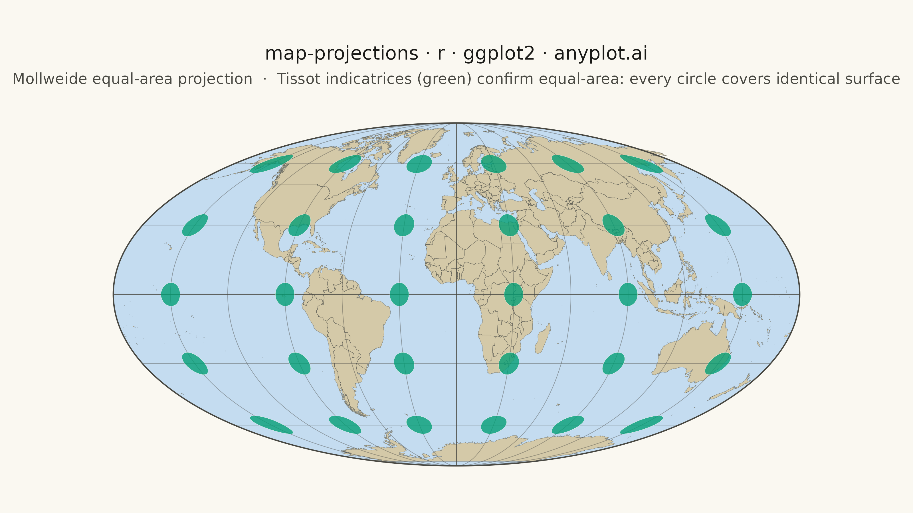
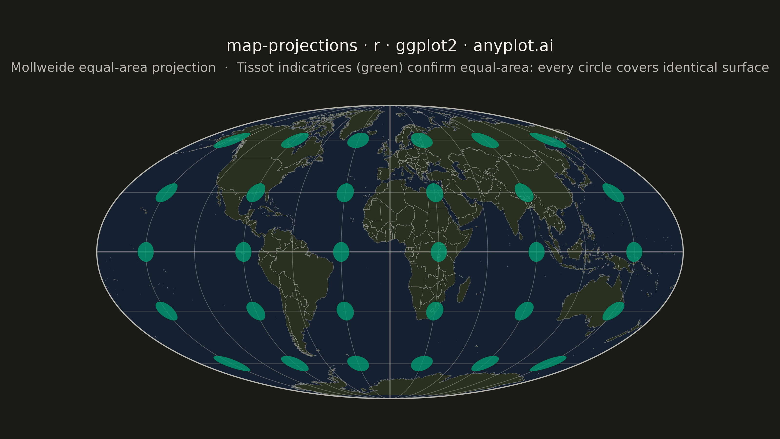
A world map demonstrating different cartographic projections and their distortion characteristics. This visualization showcases how the same geographic data appears under various map projections (Mercator, Robinson, Mollweide, Orthographic, etc.), revealing how each projection preserves or distorts area, shape, distance, or direction. The plot includes graticule (latitude/longitude grid lines) and optionally Tissot indicatrices to illustrate projection distortion patterns.
#' anyplot.ai
#' map-projections: World Map with Different Projections
#' Library: ggplot2 3.5.1 | R 4.4.1
#' Quality: 85/100 | Created: 2026-05-23

library(ggplot2)
library(maps)
library(ragg)

# Theme tokens
THEME       <- Sys.getenv("ANYPLOT_THEME", "light")
PAGE_BG     <- if (THEME == "light") "#FAF8F1" else "#1A1A17"
INK         <- if (THEME == "light") "#1A1A17" else "#F0EFE8"
INK_SOFT    <- if (THEME == "light") "#4A4A44" else "#B8B7B0"
OCEAN_BG    <- if (THEME == "light") "#C4DCF0" else "#152030"
LAND_BG     <- if (THEME == "light") "#D4C9A8" else "#2A3020"

IMPRINT <- c(
    "#009E73", "#C475FD", "#AE3030", "#4467A3",
    "#99B314", "#954477", "#BD8233"
)

# --- Mollweide projection math -----------------------------------------------
# Solve 2*theta + sin(2*theta) = pi*sin(lat) via Newton-Raphson
solve_theta <- function(phi_vec) {
    sapply(phi_vec, function(p) {
        if (is.na(p)) return(NA_real_)
        if (abs(p) >= pi / 2 - 1e-9) return(sign(p) * pi / 2)
        t <- p
        for (i in seq_len(60)) {
            delta <- (2 * t + sin(2 * t) - pi * sin(p)) / (2 + 2 * cos(2 * t))
            t     <- t - delta
            if (abs(delta) < 1e-11) break
        }
        t
    })
}

mollweide <- function(lon_deg, lat_deg) {
    lon   <- lon_deg * pi / 180
    lat   <- lat_deg * pi / 180
    theta <- solve_theta(lat)
    data.frame(
        x = (2 * sqrt(2) / pi) * lon * cos(theta),
        y = sqrt(2) * sin(theta)
    )
}

# --- World country boundaries (projected) ------------------------------------
world      <- map_data("world")
world_proj <- mollweide(world$long, world$lat)
world$x    <- world_proj$x
world$y    <- world_proj$y

# --- Projection boundary (Mollweide ellipse: a=2√2, b=√2) -------------------
t_ell    <- seq(0, 2 * pi, length.out = 721)
boundary <- data.frame(
    x = 2 * sqrt(2) * cos(t_ell),
    y = sqrt(2) * sin(t_ell)
)

# --- Graticule (lat/lon grid at 30° intervals) --------------------------------
lat_dense <- seq(-90,  90,  length.out = 541)
lon_dense <- seq(-180, 180, length.out = 1081)

meridians <- do.call(rbind, lapply(seq(-180, 180, by = 30), function(lon0) {
    pts <- mollweide(rep(lon0, length(lat_dense)), lat_dense)
    data.frame(x = pts$x, y = pts$y, group = paste0("mer_", lon0))
}))

parallels <- do.call(rbind, lapply(seq(-90, 90, by = 30), function(lat0) {
    pts <- mollweide(lon_dense, rep(lat0, length(lon_dense)))
    data.frame(x = pts$x, y = pts$y, group = paste0("par_", lat0))
}))

graticule <- rbind(meridians, parallels)

# --- Tissot indicatrices (small geodesic circles on the sphere) ---------------
# Radius in degrees; longitude offset corrected for latitude (cos projection)
r_deg    <- 5
t_circle <- seq(0, 2 * pi, length.out = 73)   # 73 pts → closed polygon

lat_centers <- seq(-60, 60, by = 30)   # 5 latitude bands
lon_centers <- seq(-150, 150, by = 60) # 6 longitude positions

tissot <- do.call(rbind, lapply(lat_centers, function(lat0) {
    cos_lat <- max(cos(lat0 * pi / 180), 0.08)
    do.call(rbind, lapply(lon_centers, function(lon0) {
        lon_c <- lon0 + r_deg * cos(t_circle) / cos_lat
        lat_c <- pmax(pmin(lat0 + r_deg * sin(t_circle), 89.9), -89.9)
        pts   <- mollweide(lon_c, lat_c)
        data.frame(
            x     = pts$x,
            y     = pts$y,
            group = paste0("t_", lon0, "_", lat0)
        )
    }))
}))

# --- Equator and prime meridian highlights -----------------------------------
equator <- mollweide(lon_dense, rep(0, length(lon_dense)))
equator$group <- "equator"

prime_merid <- mollweide(rep(0, length(lat_dense)), lat_dense)
prime_merid$group <- "prime"

# --- Plot --------------------------------------------------------------------
p <- ggplot() +
    # Ocean fill
    geom_polygon(
        data = boundary, aes(x = x, y = y),
        fill = OCEAN_BG, color = NA
    ) +
    # Land masses (country polygons)
    geom_polygon(
        data = world, aes(x = x, y = y, group = group),
        fill = LAND_BG, color = NA
    ) +
    # Country borders / coastlines
    geom_path(
        data = world, aes(x = x, y = y, group = group),
        color = INK_SOFT, linewidth = 0.10, alpha = 0.55
    ) +
    # Standard graticule (30° grid)
    geom_path(
        data = graticule, aes(x = x, y = y, group = group),
        color = INK_SOFT, linewidth = 0.18, alpha = 0.45
    ) +
    # Equator and prime meridian — slightly bolder
    geom_path(
        data = equator, aes(x = x, y = y, group = group),
        color = INK_SOFT, linewidth = 0.35, alpha = 0.70
    ) +
    geom_path(
        data = prime_merid, aes(x = x, y = y, group = group),
        color = INK_SOFT, linewidth = 0.35, alpha = 0.70
    ) +
    # Tissot indicatrices — anyplot brand green (position 1)
    geom_polygon(
        data = tissot, aes(x = x, y = y, group = group),
        fill = IMPRINT[1], color = PAGE_BG,
        linewidth = 0.06, alpha = 0.78
    ) +
    # Ellipse outline
    geom_path(
        data = boundary, aes(x = x, y = y),
        color = INK_SOFT, linewidth = 0.40
    ) +
    coord_fixed() +
    labs(
        title    = "map-projections · r · ggplot2 · anyplot.ai",
        subtitle = "Mollweide equal-area projection  ·  Tissot indicatrices (green) confirm equal-area: every circle covers identical surface"
    ) +
    theme_void(base_size = 8) +
    theme(
        plot.background = element_rect(fill = PAGE_BG, color = PAGE_BG),
        plot.title      = element_text(
            color  = INK, size = 12, hjust = 0.5,
            margin = margin(t = 14, b = 6)
        ),
        plot.subtitle   = element_text(
            color  = INK_SOFT, size = 9.5, hjust = 0.5,
            margin = margin(b = 12)
        ),
        plot.margin     = margin(8, 50, 12, 50)
    )

# --- Save --------------------------------------------------------------------
ggsave(
    filename = sprintf("plot-%s.png", THEME),
    plot     = p,
    device   = ragg::agg_png,
    width    = 8,
    height   = 4.5,
    units    = "in",
    dpi      = 400
)
Runnable source as JSON, for any HTTP client: https://api.anyplot.ai/specs/map-projections/ggplot2/code. Any spec id and library id listed in llms-full.txt fit the same URL shape; every URL below is complete and callable.
{
  "spec_id": "map-projections",
  "language": "r",
  "library": "ggplot2",
  "page": "https://anyplot.ai/map-projections/r/ggplot2",
  "hub": "https://anyplot.ai/map-projections",
  "code_json": "https://api.anyplot.ai/specs/map-projections/ggplot2/code",
  "spec_json": "https://api.anyplot.ai/specs/map-projections",
  "render_light_png": "https://storage.googleapis.com/anyplot-images/plots/map-projections/r/ggplot2/plot-light.png",
  "render_dark_png": "https://storage.googleapis.com/anyplot-images/plots/map-projections/r/ggplot2/plot-dark.png",
  "quality_score": 85.0,
  "license": "MIT",
  "guide": "https://anyplot.ai/llms.txt"
}
Part of World Map with Different Projections on anyplot.ai.