The same plot in 14 other libraries — Python: Altair, Bokeh, lets-plot, Matplotlib, Plotly, plotnine, Pygal, Seaborn; Julia: Makie.jl; JavaScript: Chart.js, D3.js, Apache ECharts, Highcharts, MUI X Charts. Compare all 15 side by side: Partial Dependence Plot in Python, R, Julia and JavaScript.
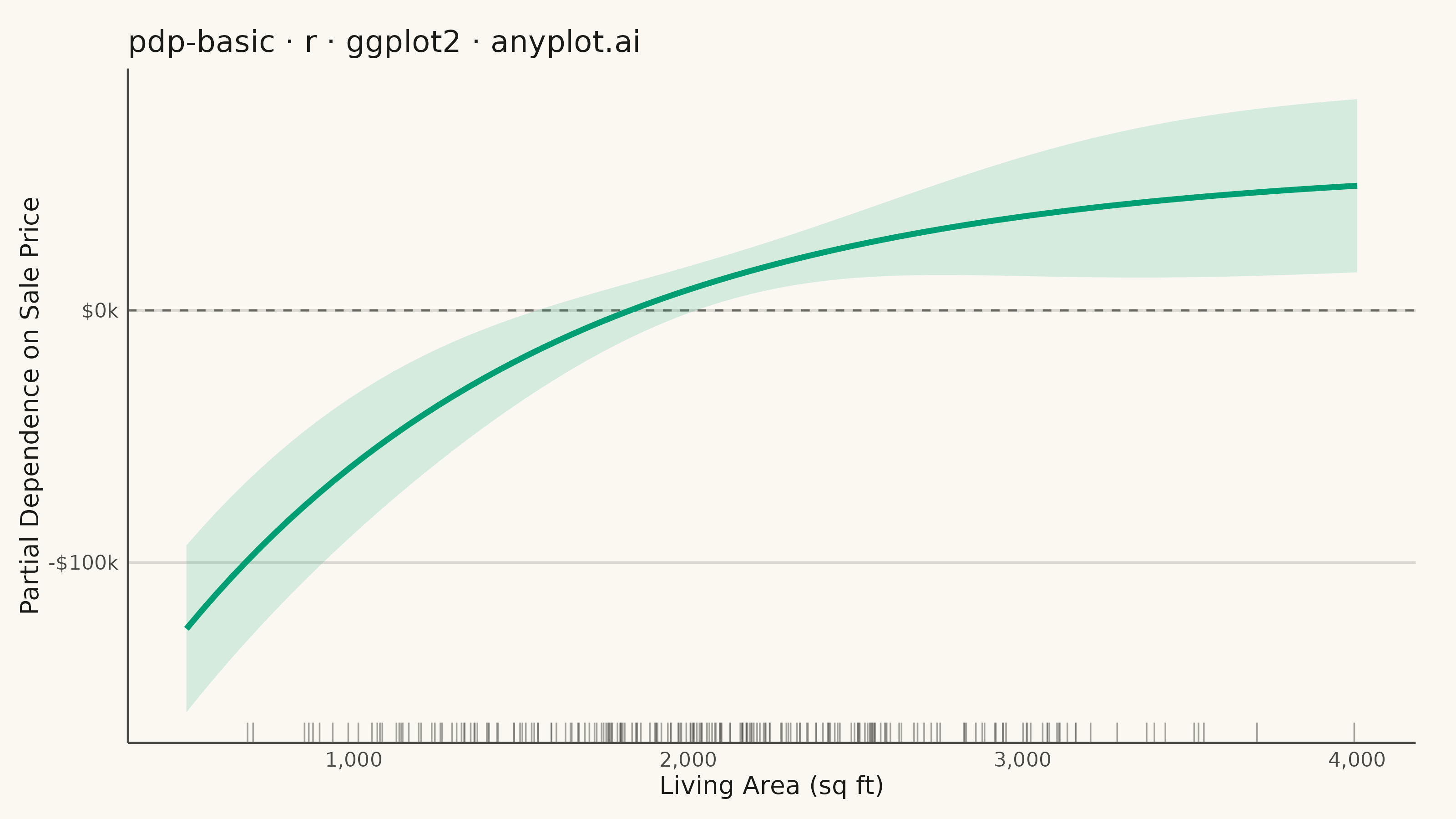
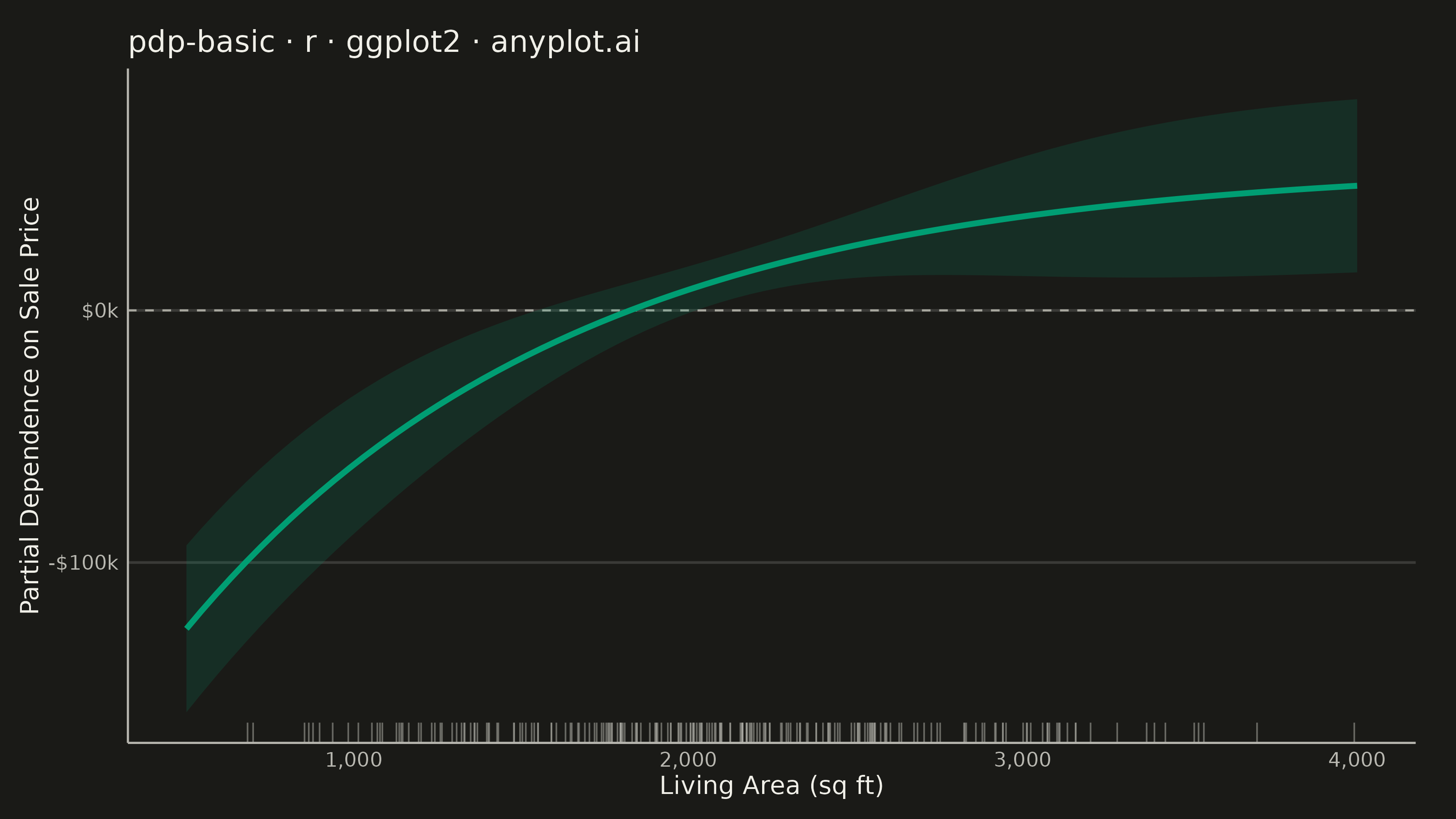
A partial dependence plot (PDP) showing the marginal effect of one feature on the predicted outcome of a machine learning model. The plot displays how predictions change as a feature varies across its range, while averaging over the effects of all other features. This visualization is essential for understanding the relationship between individual features and model predictions in interpretable machine learning.
#' anyplot.ai
#' pdp-basic: Partial Dependence Plot
#' Library: ggplot2 3.5.1 | R 4.4.1
#' Quality: 94/100 | Created: 2026-09-05

library(ggplot2)
library(tibble)
library(scales)
library(ragg)

set.seed(42)

# --- Theme tokens -------------------------------------------------------
THEME     <- Sys.getenv("ANYPLOT_THEME", "light")
PAGE_BG   <- if (THEME == "light") "#FAF8F1" else "#1A1A17"
INK       <- if (THEME == "light") "#1A1A17" else "#F0EFE8"
INK_SOFT  <- if (THEME == "light") "#4A4A44" else "#B8B7B0"
INK_MUTED <- if (THEME == "light") "#6B6A63" else "#A8A79F"
GRID      <- adjustcolor(INK, alpha.f = 0.15)
IMPRINT_PALETTE <- c(
  "#009E73", "#C475FD", "#4467A3", "#BD8233",
  "#AE3030", "#2ABCCD", "#954477", "#99B314"
)
BRAND <- IMPRINT_PALETTE[1]

# --- Data -----------------------------------------------------------------
# Partial dependence of a gradient boosting regressor predicting house sale
# price from living area (sq ft), averaging over every other feature.
living_area <- seq(500, 4000, length.out = 80)

# Diminishing marginal effect of extra square footage, centered at zero so
# the curve reads as a relative price effect rather than an absolute level.
raw_effect <- 285000 * (1 - exp(-living_area / 1150))
partial_dependence <- raw_effect - mean(raw_effect)

# Model uncertainty widens where training data thins out at the tails.
density_weight <- dnorm(living_area, mean = 2100, sd = 700)
band_halfwidth <- 9000 + 26000 * (1 - density_weight / max(density_weight))

pdp_df <- tibble(
  living_area        = living_area,
  partial_dependence = partial_dependence,
  lower              = partial_dependence - band_halfwidth,
  upper              = partial_dependence + band_halfwidth
)

# Observed training values for the rug, drawn from the same density that
# shaped the uncertainty band above.
rug_values <- rnorm(220, mean = 2100, sd = 700)
rug_df <- tibble(living_area = rug_values[rug_values >= 500 & rug_values <= 4000])

# --- Plot -------------------------------------------------------------------
p <- ggplot(pdp_df, aes(x = living_area, y = partial_dependence)) +
  geom_hline(yintercept = 0, color = INK_MUTED, linewidth = 0.4, linetype = "dashed") +
  geom_ribbon(aes(ymin = lower, ymax = upper), fill = BRAND, alpha = 0.15) +
  geom_line(color = BRAND, linewidth = 1.1) +
  geom_rug(
    data = rug_df, aes(x = living_area), inherit.aes = FALSE,
    sides = "b", color = INK_SOFT, alpha = 0.5, linewidth = 0.3
  ) +
  scale_x_continuous(labels = scales::comma) +
  scale_y_continuous(labels = scales::dollar_format(scale = 1e-3, suffix = "k")) +
  labs(
    title = "pdp-basic · r · ggplot2 · anyplot.ai",
    x     = "Living Area (sq ft)",
    y     = "Partial Dependence on Sale Price"
  ) +
  theme_minimal(base_size = 8) +
  theme(
    plot.background     = element_rect(fill = PAGE_BG, color = PAGE_BG),
    panel.background    = element_rect(fill = PAGE_BG, color = NA),
    panel.grid.major.y  = element_line(color = GRID, linewidth = 0.5),
    panel.grid.minor    = element_blank(),
    panel.grid.major.x  = element_blank(),
    axis.line           = element_line(color = INK_SOFT, linewidth = 0.4),
    axis.ticks          = element_blank(),
    axis.title          = element_text(color = INK, size = 10),
    axis.text           = element_text(color = INK_SOFT, size = 8),
    plot.title          = element_text(color = INK, size = 12),
    plot.margin         = margin(12, 16, 8, 8)
  )

# --- Save -------------------------------------------------------------------
ggsave(
  filename = sprintf("plot-%s.png", THEME),
  plot     = p,
  device   = ragg::agg_png,
  width    = 8,
  height   = 4.5,
  units    = "in",
  dpi      = 400
)
Runnable source as JSON, for any HTTP client: https://api.anyplot.ai/specs/pdp-basic/ggplot2/code. Any spec id and library id listed in llms-full.txt fit the same URL shape; every URL below is complete and callable.
{
  "spec_id": "pdp-basic",
  "language": "r",
  "library": "ggplot2",
  "page": "https://anyplot.ai/pdp-basic/r/ggplot2",
  "hub": "https://anyplot.ai/pdp-basic",
  "code_json": "https://api.anyplot.ai/specs/pdp-basic/ggplot2/code",
  "spec_json": "https://api.anyplot.ai/specs/pdp-basic",
  "render_light_png": "https://storage.googleapis.com/anyplot-images/plots/pdp-basic/r/ggplot2/plot-light.png",
  "render_dark_png": "https://storage.googleapis.com/anyplot-images/plots/pdp-basic/r/ggplot2/plot-dark.png",
  "quality_score": 94.0,
  "license": "MIT",
  "guide": "https://anyplot.ai/llms.txt"
}
Part of Partial Dependence Plot on anyplot.ai.