The same plot in 14 other libraries — JavaScript: Chart.js, Apache ECharts, Highcharts, MUI X Charts; Python: Altair, Bokeh, lets-plot, Matplotlib, Plotly, plotnine, Pygal, Seaborn; R: ggplot2; Julia: Makie.jl. Compare all 15 side by side: Phase Diagram (State Space Plot) in Python, R, Julia and JavaScript.
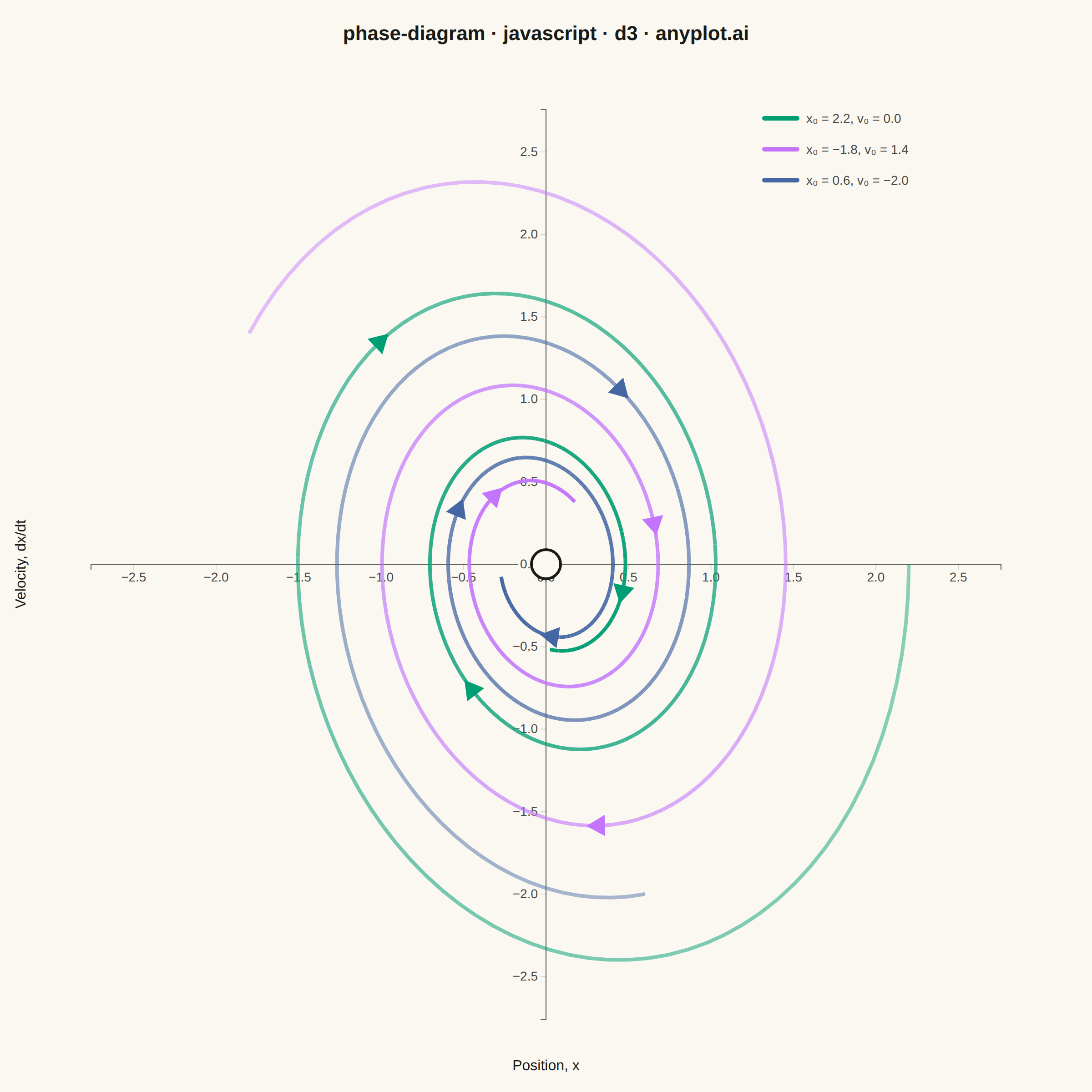
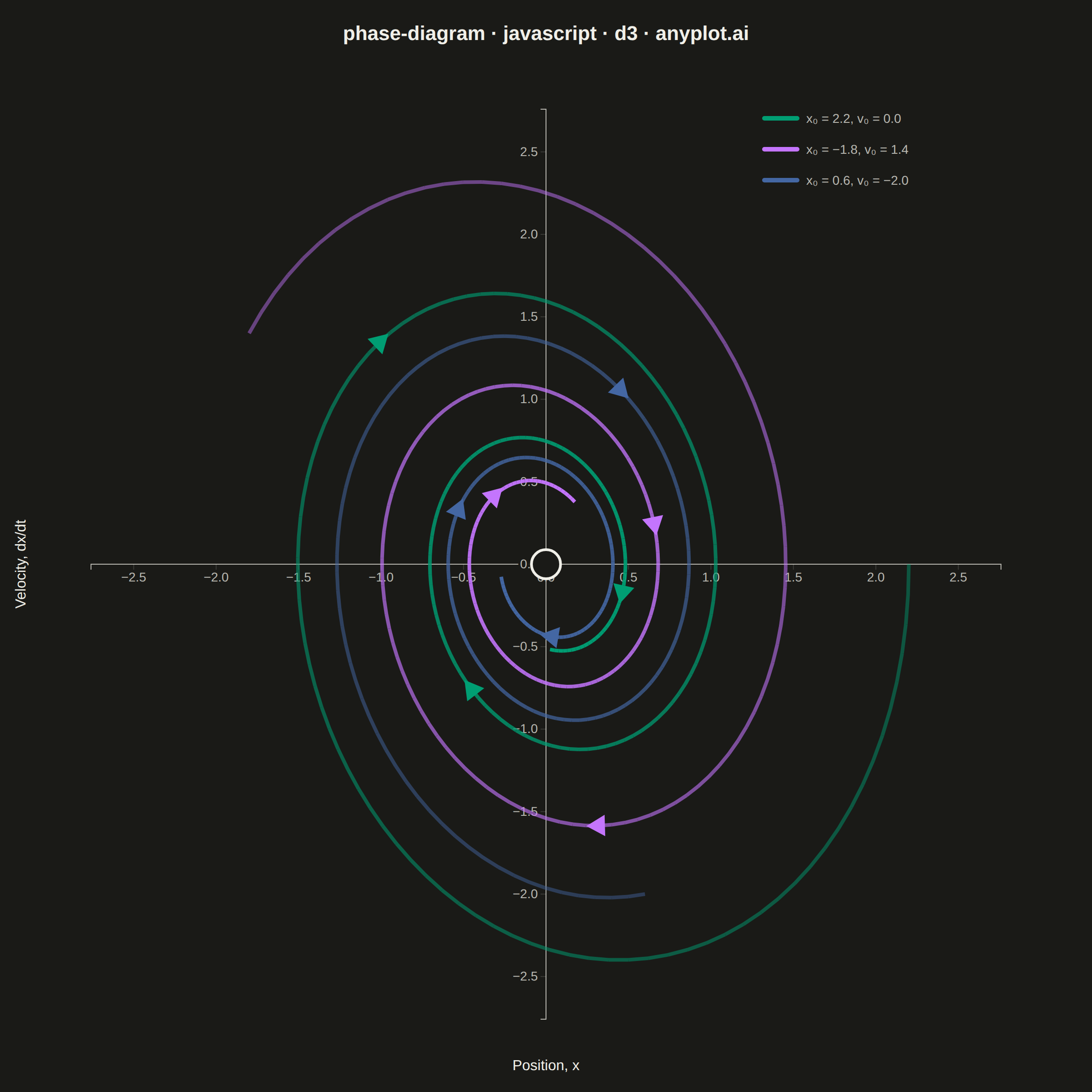
A phase diagram (or state space plot) displays the trajectory of a dynamical system by plotting a variable against its derivative (x vs dx/dt). This visualization reveals the qualitative behavior of systems including fixed points, limit cycles, stability, and oscillation patterns. It is essential for analyzing differential equations without solving them explicitly.
// anyplot.ai
// phase-diagram: Phase Diagram (State Space Plot)
// Library: d3 7.9.0 | JavaScript 22.23.2
// Quality: 87/100 | Created: 2026-09-05

//# anyplot-orientation: square
const t = window.ANYPLOT_TOKENS;
const { width, height } = window.ANYPLOT_SIZE;
const margin = { top: 120, right: 100, bottom: 80, left: 100 };
const iw = width - margin.left - margin.right;
const ih = height - margin.top - margin.bottom;

// --- Physics: damped harmonic oscillator ------------------------------------
// dx/dt = v ; dv/dt = -2*zeta*omega*v - omega^2*x  (RK4, fixed-seed deterministic)
const OMEGA = 1.3;
const ZETA = 0.12;
const DT = 0.05;
const STEPS = 220;

function derivative(state) {
  const [x, v] = state;
  return [v, -2 * ZETA * OMEGA * v - OMEGA * OMEGA * x];
}

function rk4Step(state, dt) {
  const k1 = derivative(state);
  const k2 = derivative([state[0] + (dt / 2) * k1[0], state[1] + (dt / 2) * k1[1]]);
  const k3 = derivative([state[0] + (dt / 2) * k2[0], state[1] + (dt / 2) * k2[1]]);
  const k4 = derivative([state[0] + dt * k3[0], state[1] + dt * k3[1]]);
  return [
    state[0] + (dt / 6) * (k1[0] + 2 * k2[0] + 2 * k3[0] + k4[0]),
    state[1] + (dt / 6) * (k1[1] + 2 * k2[1] + 2 * k3[1] + k4[1]),
  ];
}

function integrate(x0, v0, dt, steps) {
  const points = [{ x: x0, v: v0 }];
  let state = [x0, v0];
  for (let i = 0; i < steps; i++) {
    state = rk4Step(state, dt);
    points.push({ x: state[0], v: state[1] });
  }
  return points;
}

// --- Data: three initial conditions spiraling into the stable fixed point --
const initialConditions = [
  { x0: 2.2, v0: 0.0, label: "x₀ = 2.2, v₀ = 0.0" },
  { x0: -1.8, v0: 1.4, label: "x₀ = −1.8, v₀ = 1.4" },
  { x0: 0.6, v0: -2.0, label: "x₀ = 0.6, v₀ = −2.0" },
];
const trajectories = initialConditions.map((ic, i) => ({
  ...ic,
  color: t.palette[i],
  points: integrate(ic.x0, ic.v0, DT, STEPS),
}));

const allValues = trajectories.flatMap((tr) => tr.points.flatMap((p) => [p.x, p.v]));
const maxAbs = d3.max(allValues, (v) => Math.abs(v)) * 1.15;

// --- SVG mount + scales (equal domain span on both axes keeps spirals
//     geometrically correct instead of visually stretched) ------------------
const svg = d3.select("#container").append("svg").attr("width", width).attr("height", height);
const g = svg.append("g").attr("transform", `translate(${margin.left},${margin.top})`);

const x = d3.scaleLinear().domain([-maxAbs, maxAbs]).range([0, iw]);
const v = d3.scaleLinear().domain([-maxAbs, maxAbs]).range([ih, 0]);

// --- Axes crossing at the origin (the fixed point) --------------------------
const xAxisG = g.append("g").attr("transform", `translate(0,${v(0)})`).call(d3.axisBottom(x).ticks(8));
const yAxisG = g.append("g").attr("transform", `translate(${x(0)},0)`).call(d3.axisLeft(v).ticks(8));
for (const ax of [xAxisG, yAxisG]) {
  // Origin-crossing ticks sit inside the densest trajectory overlap, so give
  // the labels a page-colored halo (paint-order stroke) to stay legible
  // instead of competing with the spiral strokes underneath.
  ax.selectAll("text")
    .attr("fill", t.inkSoft)
    .style("font-size", "14px")
    .style("paint-order", "stroke")
    .style("stroke", t.pageBg)
    .style("stroke-width", "5px")
    .style("stroke-linejoin", "round");
  ax.selectAll("line").attr("stroke", t.grid);
  ax.select(".domain").attr("stroke", t.inkSoft);
}

// --- Trajectories: opacity ramps with elapsed time, arrowheads show flow ---
// Each RK4 step is drawn as its own butt-capped segment (no shared-endpoint
// overlap between adjacent segments) so the per-step opacity ramp reads as a
// smooth fade instead of banding at chunk boundaries.
for (const tr of trajectories) {
  const n = tr.points.length;
  for (let i = 0; i < n - 1; i++) {
    const opacity = 0.45 + 0.55 * (i / (n - 2));
    g.append("line")
      .attr("x1", x(tr.points[i].x))
      .attr("y1", v(tr.points[i].v))
      .attr("x2", x(tr.points[i + 1].x))
      .attr("y2", v(tr.points[i + 1].v))
      .attr("stroke", tr.color)
      .attr("stroke-width", 4)
      .attr("stroke-linecap", "butt")
      .attr("opacity", opacity);
  }

  const arrowTriangle = d3.symbol().type(d3.symbolTriangle).size(240)();
  for (const frac of [0.28, 0.6, 0.9]) {
    const i = Math.min(n - 2, Math.max(1, Math.round(frac * n)));
    const before = tr.points[i - 1];
    const after = tr.points[i + 1];
    const dx = x(after.x) - x(before.x);
    const dy = v(after.v) - v(before.v);
    const angle = (Math.atan2(dy, dx) * 180) / Math.PI + 90;
    g.append("path")
      .attr("d", arrowTriangle)
      .attr("transform", `translate(${x(tr.points[i].x)},${v(tr.points[i].v)}) rotate(${angle})`)
      .attr("fill", tr.color);
  }
}

// --- Fixed point marker (stable equilibrium at the origin) ------------------
g.append("circle")
  .attr("cx", x(0))
  .attr("cy", v(0))
  .attr("r", 16)
  .attr("fill", t.pageBg)
  .attr("stroke", t.ink)
  .attr("stroke-width", 3);

// --- Legend (initial conditions) --------------------------------------------
const legendX = iw - 260;
const legendY = 10;
trajectories.forEach((tr, i) => {
  const ly = legendY + i * 34;
  g.append("line")
    .attr("x1", legendX)
    .attr("x2", legendX + 36)
    .attr("y1", ly)
    .attr("y2", ly)
    .attr("stroke", tr.color)
    .attr("stroke-width", 5)
    .attr("stroke-linecap", "round");
  g.append("text")
    .attr("x", legendX + 46)
    .attr("y", ly + 5)
    .attr("fill", t.inkSoft)
    .style("font-size", "14px")
    .text(tr.label);
});

// --- Axis labels --------------------------------------------------------------
svg
  .append("text")
  .attr("x", margin.left + iw / 2)
  .attr("y", height - 24)
  .attr("text-anchor", "middle")
  .attr("fill", t.ink)
  .style("font-size", "16px")
  .text("Position, x");

svg
  .append("text")
  .attr("transform", `translate(28,${margin.top + ih / 2}) rotate(-90)`)
  .attr("text-anchor", "middle")
  .attr("fill", t.ink)
  .style("font-size", "16px")
  .text("Velocity, dx/dt");

// --- Title -------------------------------------------------------------------
svg
  .append("text")
  .attr("x", width / 2)
  .attr("y", 44)
  .attr("text-anchor", "middle")
  .attr("fill", t.ink)
  .style("font-size", "22px")
  .style("font-weight", "600")
  .text("phase-diagram · javascript · d3 · anyplot.ai");
Runnable source as JSON, for any HTTP client: https://api.anyplot.ai/specs/phase-diagram/d3/code. Any spec id and library id listed in llms-full.txt fit the same URL shape; every URL below is complete and callable.
{
  "spec_id": "phase-diagram",
  "language": "javascript",
  "library": "d3",
  "page": "https://anyplot.ai/phase-diagram/javascript/d3",
  "hub": "https://anyplot.ai/phase-diagram",
  "code_json": "https://api.anyplot.ai/specs/phase-diagram/d3/code",
  "spec_json": "https://api.anyplot.ai/specs/phase-diagram",
  "render_light_png": "https://storage.googleapis.com/anyplot-images/plots/phase-diagram/javascript/d3/plot-light.png",
  "render_dark_png": "https://storage.googleapis.com/anyplot-images/plots/phase-diagram/javascript/d3/plot-dark.png",
  "interactive_light_html": "https://storage.googleapis.com/anyplot-images/plots/phase-diagram/javascript/d3/plot-light.html",
  "interactive_dark_html": "https://storage.googleapis.com/anyplot-images/plots/phase-diagram/javascript/d3/plot-dark.html",
  "quality_score": 87.0,
  "license": "MIT",
  "guide": "https://anyplot.ai/llms.txt"
}
Part of Phase Diagram (State Space Plot) on anyplot.ai.