The same plot in 14 other libraries — Python: Altair, Bokeh, lets-plot, Matplotlib, Plotly, plotnine, Pygal, Seaborn; R: ggplot2; JavaScript: Chart.js, D3.js, Apache ECharts, Highcharts, MUI X Charts. Compare all 15 side by side: Phase Diagram (State Space Plot) in Python, R, Julia and JavaScript.
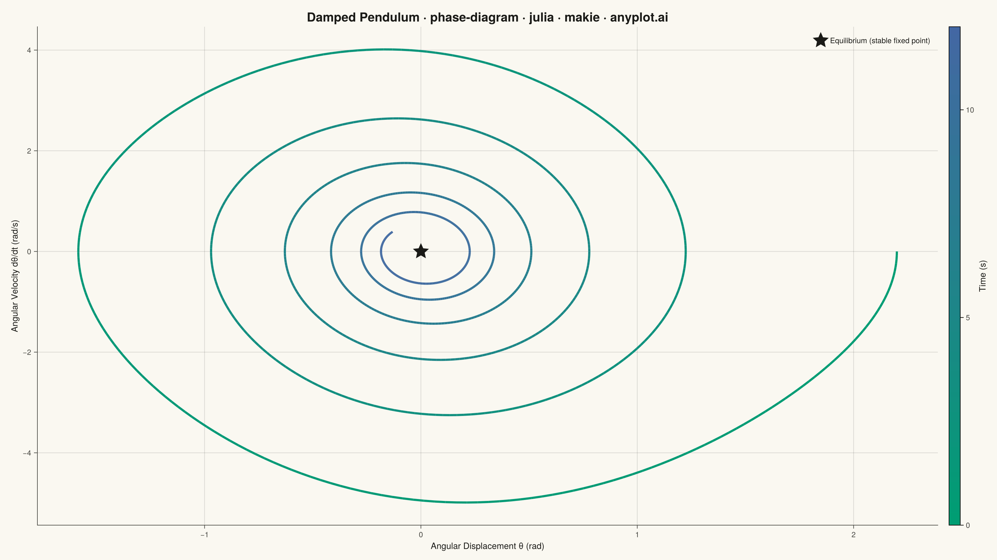
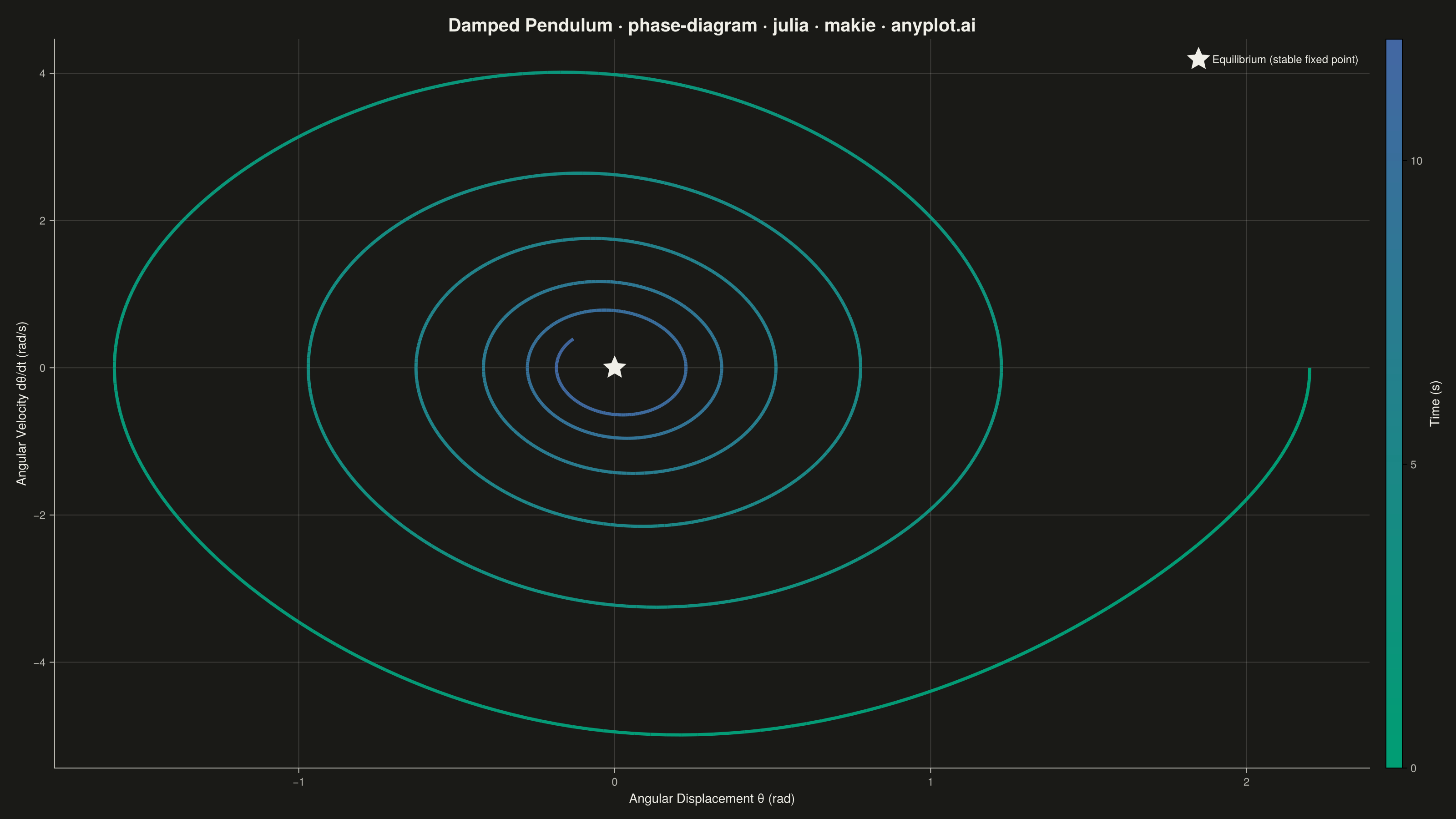
A phase diagram (or state space plot) displays the trajectory of a dynamical system by plotting a variable against its derivative (x vs dx/dt). This visualization reveals the qualitative behavior of systems including fixed points, limit cycles, stability, and oscillation patterns. It is essential for analyzing differential equations without solving them explicitly.
# anyplot.ai
# phase-diagram: Phase Diagram (State Space Plot)
# Library: makie 0.21.9 | Julia 1.11.9
# Quality: 91/100 | Created: 2026-09-05

using CairoMakie
using Colors
using ColorSchemes
using Random

Random.seed!(42)

# --- Theme tokens ------------------------------------------------------------
const THEME       = get(ENV, "ANYPLOT_THEME", "light")
const PAGE_BG     = THEME == "light" ? colorant"#FAF8F1" : colorant"#1A1A17"
const ELEVATED_BG = THEME == "light" ? colorant"#FFFDF6" : colorant"#242420"
const INK         = THEME == "light" ? colorant"#1A1A17" : colorant"#F0EFE8"
const INK_SOFT    = THEME == "light" ? colorant"#4A4A44" : colorant"#B8B7B0"

# Continuous data (elapsed time) — sequential Imprint cmap, single polarity
const ANYPLOT_SEQ = cgrad([colorant"#009E73", colorant"#4467A3"])

# --- Data: damped pendulum trajectory (RK4 integration) ----------------------
# theta'' + damping * theta' + (gravity / arm_length) * sin(theta) = 0
gravity = 9.81
arm_length = 1.0
damping = 0.4
dt = 0.01
n_steps = 1200

theta = zeros(n_steps + 1)
omega = zeros(n_steps + 1)
elapsed = zeros(n_steps + 1)
theta[1] = 2.2
omega[1] = 0.0

for i in 1:n_steps
    th = theta[i]
    om = omega[i]

    k1_theta = om
    k1_omega = -damping * om - (gravity / arm_length) * sin(th)

    k2_theta = om + 0.5 * dt * k1_omega
    k2_omega = -damping * (om + 0.5 * dt * k1_omega) -
               (gravity / arm_length) * sin(th + 0.5 * dt * k1_theta)

    k3_theta = om + 0.5 * dt * k2_omega
    k3_omega = -damping * (om + 0.5 * dt * k2_omega) -
               (gravity / arm_length) * sin(th + 0.5 * dt * k2_theta)

    k4_theta = om + dt * k3_omega
    k4_omega = -damping * (om + dt * k3_omega) -
               (gravity / arm_length) * sin(th + dt * k3_theta)

    theta[i + 1] = th + dt / 6 * (k1_theta + 2 * k2_theta + 2 * k3_theta + k4_theta)
    omega[i + 1] = om + dt / 6 * (k1_omega + 2 * k2_omega + 2 * k3_omega + k4_omega)
    elapsed[i + 1] = elapsed[i] + dt
end

# --- Plot ---------------------------------------------------------------------
title_text = "Damped Pendulum · phase-diagram · julia · makie · anyplot.ai"

fig = Figure(
    size            = (1600, 900),
    fontsize        = 14,
    backgroundcolor = PAGE_BG,
)

ax = Axis(
    fig[1, 1];
    title             = title_text,
    titlesize         = 20,
    titlecolor        = INK,
    xlabel            = "Angular Displacement θ (rad)",
    ylabel            = "Angular Velocity dθ/dt (rad/s)",
    xlabelsize        = 14,
    ylabelsize        = 14,
    xlabelcolor       = INK,
    ylabelcolor       = INK,
    xticklabelsize    = 12,
    yticklabelsize    = 12,
    xticklabelcolor   = INK_SOFT,
    yticklabelcolor   = INK_SOFT,
    xtickcolor        = INK_SOFT,
    ytickcolor        = INK_SOFT,
    backgroundcolor   = PAGE_BG,
    leftspinecolor    = INK_SOFT,
    bottomspinecolor  = INK_SOFT,
    topspinevisible   = false,
    rightspinevisible = false,
    xgridcolor        = RGBAf(INK.r, INK.g, INK.b, 0.15),
    ygridcolor        = RGBAf(INK.r, INK.g, INK.b, 0.15),
    xminorgridvisible = false,
    yminorgridvisible = false,
)

lines!(ax, theta, omega; color = elapsed, colormap = ANYPLOT_SEQ, linewidth = 3.5)

scatter!(
    ax, [0.0], [0.0];
    marker = :star5, markersize = 30, color = INK, strokewidth = 0,
    label = "Equilibrium (stable fixed point)",
)

Colorbar(
    fig[1, 2];
    colormap       = ANYPLOT_SEQ,
    limits         = (elapsed[1], elapsed[end]),
    label          = "Time (s)",
    labelcolor     = INK,
    labelsize      = 14,
    ticklabelsize  = 12,
    ticklabelcolor = INK_SOFT,
    width          = 18,
)

axislegend(
    ax;
    position        = :rt,
    backgroundcolor = ELEVATED_BG,
    framevisible    = false,
    labelcolor      = INK,
    labelsize       = 12,
)

# --- Save ---------------------------------------------------------------------
save("plot-$(THEME).png", fig; px_per_unit = 2)
Runnable source as JSON, for any HTTP client: https://api.anyplot.ai/specs/phase-diagram/makie/code. Any spec id and library id listed in llms-full.txt fit the same URL shape; every URL below is complete and callable.
{
  "spec_id": "phase-diagram",
  "language": "julia",
  "library": "makie",
  "page": "https://anyplot.ai/phase-diagram/julia/makie",
  "hub": "https://anyplot.ai/phase-diagram",
  "code_json": "https://api.anyplot.ai/specs/phase-diagram/makie/code",
  "spec_json": "https://api.anyplot.ai/specs/phase-diagram",
  "render_light_png": "https://storage.googleapis.com/anyplot-images/plots/phase-diagram/julia/makie/plot-light.png",
  "render_dark_png": "https://storage.googleapis.com/anyplot-images/plots/phase-diagram/julia/makie/plot-dark.png",
  "quality_score": 91.0,
  "license": "MIT",
  "guide": "https://anyplot.ai/llms.txt"
}
Part of Phase Diagram (State Space Plot) on anyplot.ai.