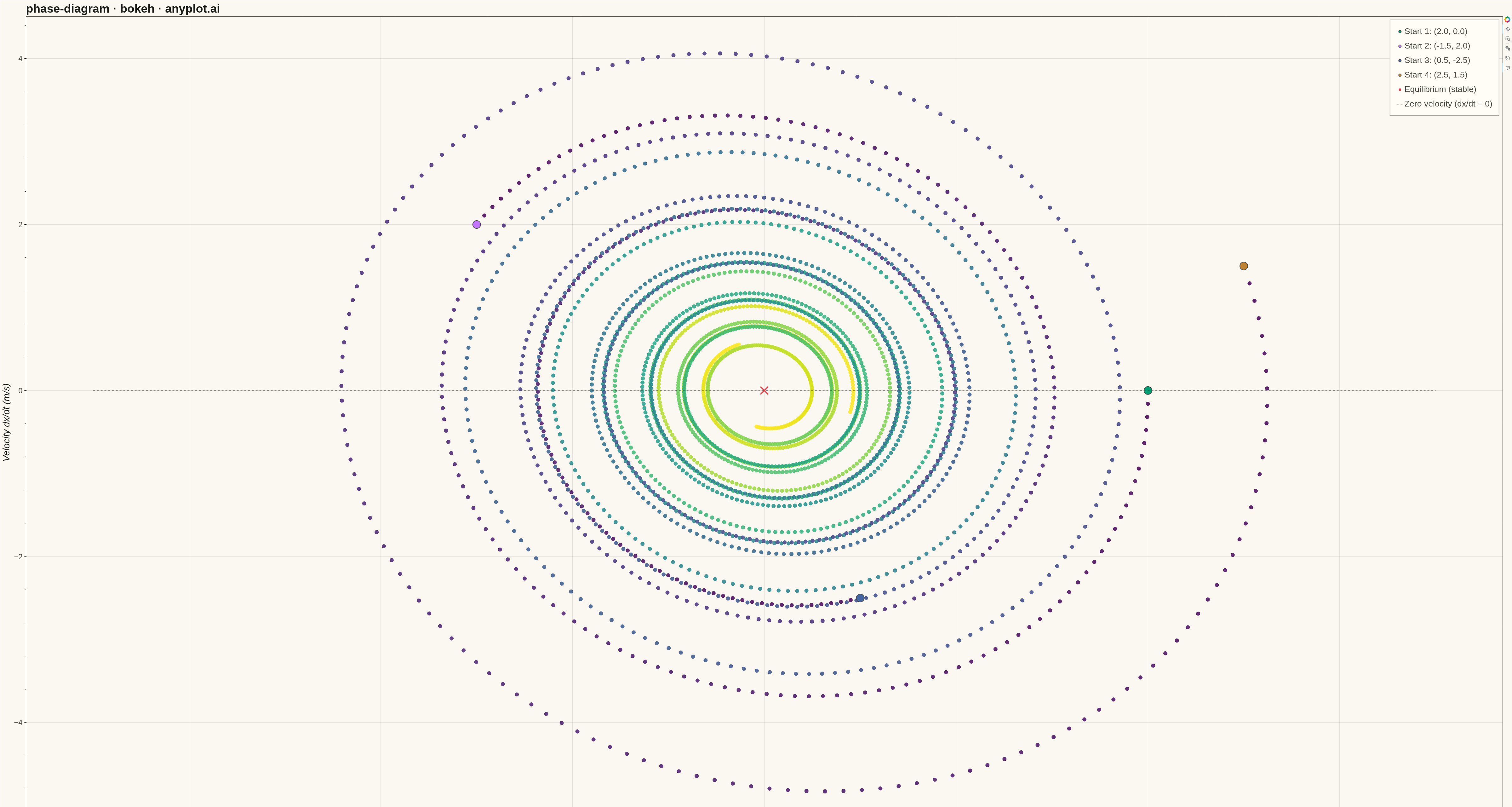
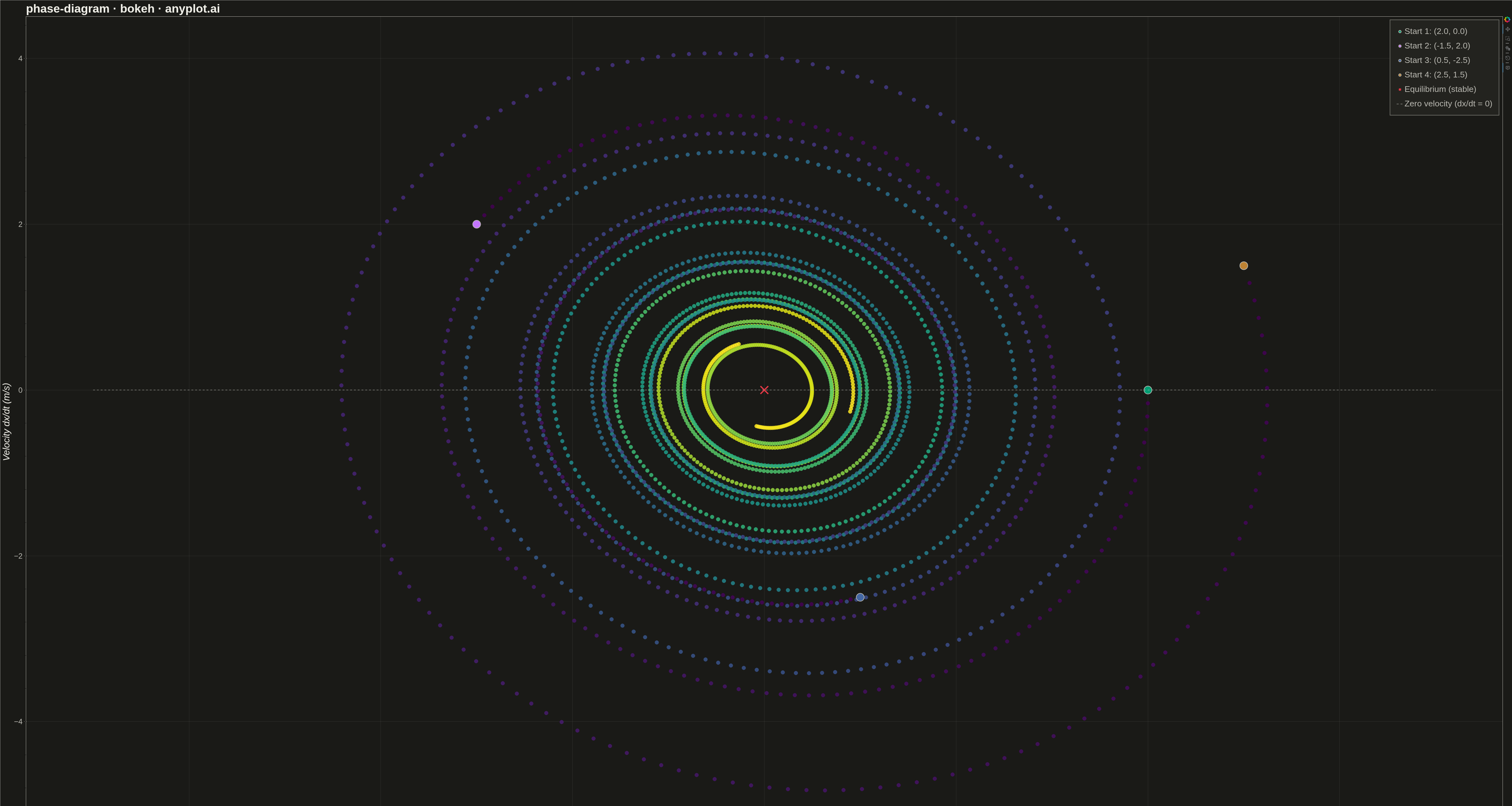
A phase diagram (or state space plot) displays the trajectory of a dynamical system by plotting a variable against its derivative (x vs dx/dt). This visualization reveals the qualitative behavior of systems including fixed points, limit cycles, stability, and oscillation patterns. It is essential for analyzing differential equations without solving them explicitly.
""" anyplot.ai
phase-diagram: Phase Diagram (State Space Plot)
Library: bokeh 3.9.0 | Python 3.13.13
Quality: 92/100 | Updated: 2026-05-14
"""

import os
import sys
import time
from pathlib import Path


script_dir = os.path.dirname(os.path.abspath(__file__))
sys.path = [p for p in sys.path if p and p != "." and p != script_dir and not p.endswith("implementations")]
os.chdir(script_dir)

import numpy as np
from bokeh.io import output_file, save
from bokeh.models import ColumnDataSource, HoverTool, LinearColorMapper
from bokeh.palettes import Viridis256
from bokeh.plotting import figure
from selenium import webdriver
from selenium.webdriver.chrome.options import Options


THEME = os.getenv("ANYPLOT_THEME", "light")
PAGE_BG = "#FAF8F1" if THEME == "light" else "#1A1A17"
ELEVATED_BG = "#FFFDF6" if THEME == "light" else "#242420"
INK = "#1A1A17" if THEME == "light" else "#F0EFE8"
INK_SOFT = "#4A4A44" if THEME == "light" else "#B8B7B0"
BRAND = "#009E73"

# Data: Damped harmonic oscillator (simple pendulum with friction)
# dx/dt = v, dv/dt = -omega^2 * x - gamma * v
np.random.seed(42)

omega = 2.0
gamma = 0.3
dt = 0.02
n_steps = 800

trajectories = []
initial_conditions = [(2.0, 0.0), (-1.5, 2.0), (0.5, -2.5), (2.5, 1.5)]

for x0, v0 in initial_conditions:
    x_traj = [x0]
    v_traj = [v0]
    t_traj = [0]
    x, v = x0, v0

    for i in range(n_steps):
        ax = -(omega**2) * x - gamma * v
        x_new = x + v * dt
        v_new = v + ax * dt
        x, v = x_new, v_new
        x_traj.append(x)
        v_traj.append(v)
        t_traj.append((i + 1) * dt)

    trajectories.append((x_traj, v_traj, t_traj))

# Create figure
p = figure(
    width=4800,
    height=2700,
    title="phase-diagram · bokeh · anyplot.ai",
    x_axis_label="Position x (displacement)",
    y_axis_label="Velocity dx/dt (m/s)",
    tools="pan,wheel_zoom,box_zoom,reset,hover",
    background_fill_color=PAGE_BG,
    border_fill_color=PAGE_BG,
)

# Theme-adaptive styling
p.title.text_font_size = "28pt"
p.title.text_color = INK
p.xaxis.axis_label_text_font_size = "22pt"
p.yaxis.axis_label_text_font_size = "22pt"
p.xaxis.axis_label_text_color = INK
p.yaxis.axis_label_text_color = INK
p.xaxis.major_label_text_font_size = "18pt"
p.yaxis.major_label_text_font_size = "18pt"
p.xaxis.major_label_text_color = INK_SOFT
p.yaxis.major_label_text_color = INK_SOFT
p.xaxis.axis_line_color = INK_SOFT
p.yaxis.axis_line_color = INK_SOFT
p.xaxis.major_tick_line_color = INK_SOFT
p.yaxis.major_tick_line_color = INK_SOFT

# Grid styling
p.xgrid.grid_line_color = INK
p.ygrid.grid_line_color = INK
p.xgrid.grid_line_alpha = 0.10
p.ygrid.grid_line_alpha = 0.10

p.outline_line_color = INK_SOFT

# Okabe-Ito colors for trajectories (first series is BRAND, then alternates)
traj_colors = [BRAND, "#C475FD", "#4467A3", "#BD8233"]

color_mapper = LinearColorMapper(palette=Viridis256, low=0, high=1)

# Plot each trajectory
for idx, (x_traj, v_traj, t_traj) in enumerate(trajectories):
    t_norm = np.array(t_traj)
    t_norm = (t_norm - t_norm.min()) / (t_norm.max() - t_norm.min())

    source = ColumnDataSource(
        data={"x": x_traj, "v": v_traj, "t_norm": t_norm.tolist(), "t": t_traj, "traj_id": [idx + 1] * len(x_traj)}
    )

    # Trajectory points with time-based coloring
    scatter = p.scatter(
        x="x", y="v", source=source, size=12, color={"field": "t_norm", "transform": color_mapper}, alpha=0.85
    )

    # Starting point marker
    p.scatter(
        x=[x_traj[0]],
        y=[v_traj[0]],
        size=25,
        color=traj_colors[idx],
        marker="circle",
        line_color=INK_SOFT,
        line_width=2,
        legend_label=f"Start {idx + 1}: ({initial_conditions[idx][0]}, {initial_conditions[idx][1]})",
    )

# Fixed point (equilibrium)
p.scatter(x=[0], y=[0], size=35, color="#E63946", marker="x", line_width=4, legend_label="Equilibrium (stable)")

# Zero velocity line
p.line(
    x=[-3.5, 3.5],
    y=[0, 0],
    line_width=2,
    line_dash="dashed",
    line_color=INK_SOFT,
    alpha=0.6,
    legend_label="Zero velocity (dx/dt = 0)",
)

# Configure HoverTool
hover = p.select_one(HoverTool)
hover.tooltips = [
    ("Position (x)", "@x{0.00}"),
    ("Velocity (dx/dt)", "@v{0.00}"),
    ("Time (s)", "@t{0.0}"),
    ("Trajectory", "@traj_id"),
]

# Legend styling
p.legend.label_text_font_size = "20pt"
p.legend.label_text_color = INK_SOFT
p.legend.location = "top_right"
p.legend.background_fill_color = ELEVATED_BG
p.legend.background_fill_alpha = 0.95
p.legend.border_line_color = INK_SOFT
p.legend.border_line_width = 2
p.legend.padding = 20
p.legend.spacing = 15

# Save HTML
output_file(f"plot-{THEME}.html")
save(p)

# Screenshot with Selenium
W, H = 4800, 2700
opts = Options()
for arg in (
    "--headless=new",
    "--no-sandbox",
    "--disable-dev-shm-usage",
    "--disable-gpu",
    f"--window-size={W},{H}",
    "--hide-scrollbars",
):
    opts.add_argument(arg)

driver = webdriver.Chrome(options=opts)
driver.set_window_size(W, H)
driver.get(f"file://{Path(f'plot-{THEME}.html').resolve()}")
time.sleep(3)
driver.save_screenshot(f"plot-{THEME}.png")
driver.quit()
Runnable source as JSON, for any HTTP client: https://api.anyplot.ai/specs/phase-diagram/bokeh/code. Any spec id and library id listed in llms-full.txt fit the same URL shape; every URL below is complete and callable.
{
  "spec_id": "phase-diagram",
  "language": "python",
  "library": "bokeh",
  "page": "https://anyplot.ai/phase-diagram/python/bokeh",
  "hub": "https://anyplot.ai/phase-diagram",
  "code_json": "https://api.anyplot.ai/specs/phase-diagram/bokeh/code",
  "spec_json": "https://api.anyplot.ai/specs/phase-diagram",
  "render_light_png": "https://storage.googleapis.com/anyplot-images/plots/phase-diagram/python/bokeh/plot-light.png",
  "render_dark_png": "https://storage.googleapis.com/anyplot-images/plots/phase-diagram/python/bokeh/plot-dark.png",
  "interactive_light_html": "https://storage.googleapis.com/anyplot-images/plots/phase-diagram/python/bokeh/plot-light.html",
  "interactive_dark_html": "https://storage.googleapis.com/anyplot-images/plots/phase-diagram/python/bokeh/plot-dark.html",
  "quality_score": 92.0,
  "license": "MIT",
  "guide": "https://anyplot.ai/llms.txt"
}
Part of Phase Diagram (State Space Plot) on anyplot.ai.