The same plot in 14 other libraries — Python: Altair, Bokeh, lets-plot, Matplotlib, Plotly, plotnine, Pygal, Seaborn; Julia: Makie.jl; JavaScript: Chart.js, D3.js, Apache ECharts, Highcharts, MUI X Charts. Compare all 15 side by side: Phase Diagram (State Space Plot) in Python, R, Julia and JavaScript.
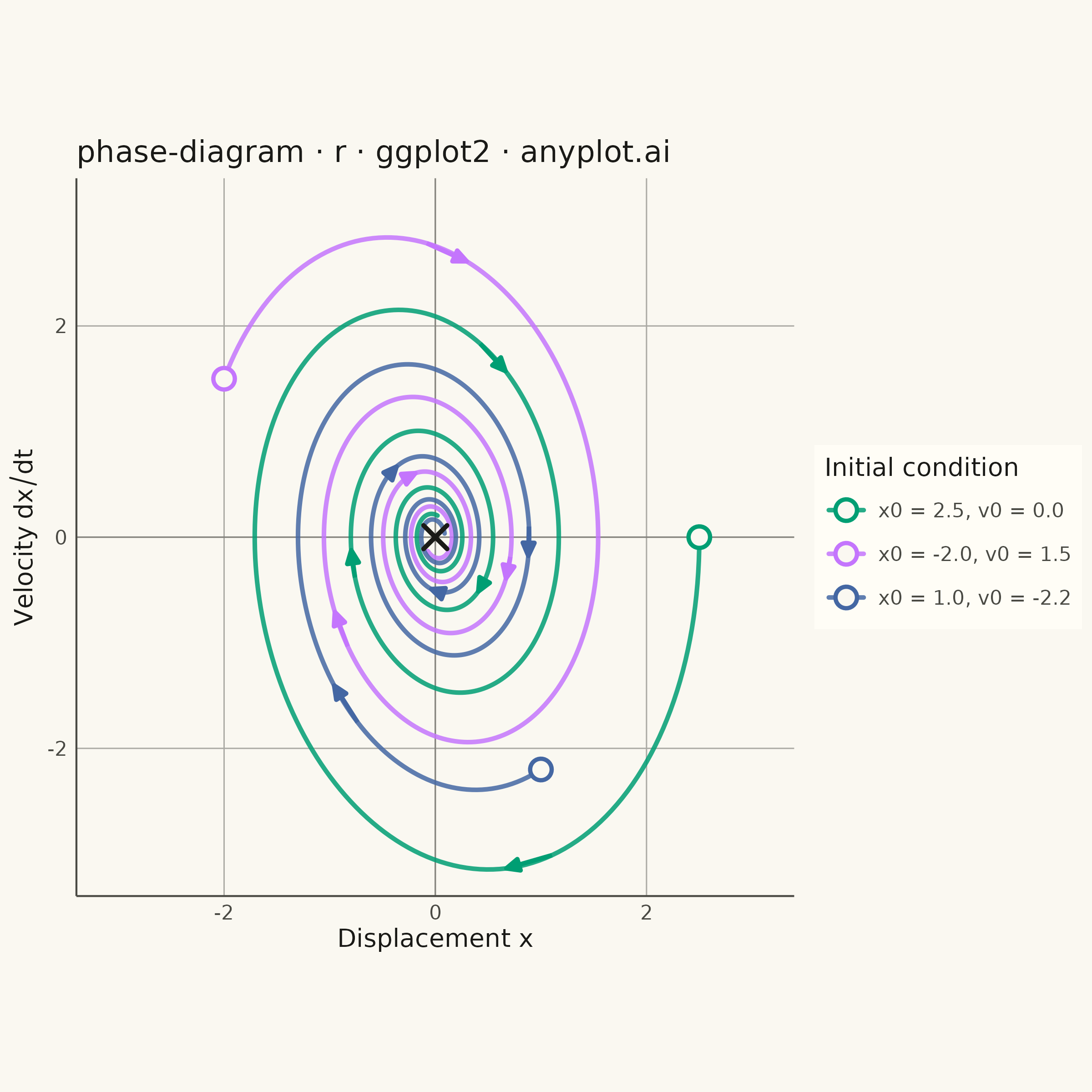
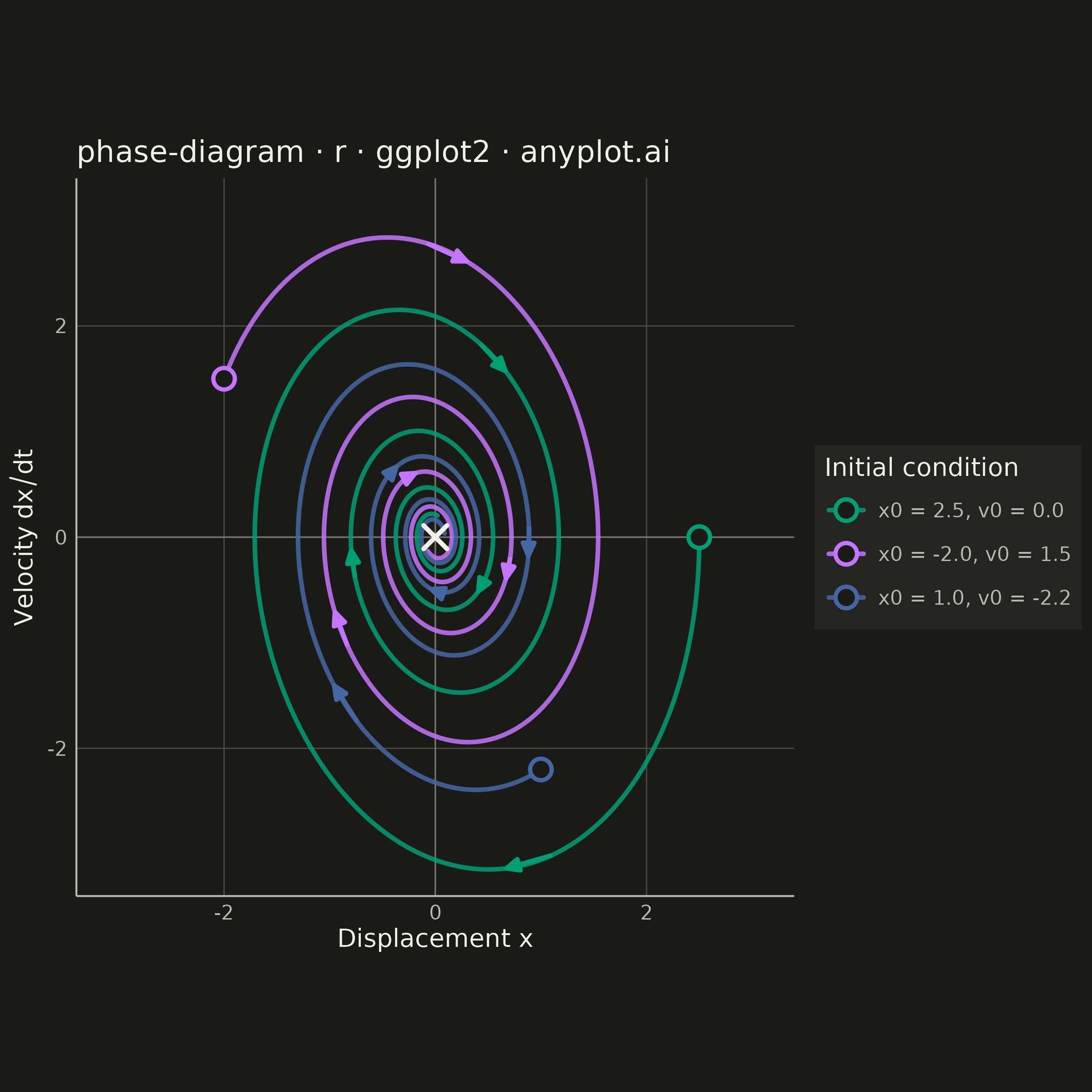
A phase diagram (or state space plot) displays the trajectory of a dynamical system by plotting a variable against its derivative (x vs dx/dt). This visualization reveals the qualitative behavior of systems including fixed points, limit cycles, stability, and oscillation patterns. It is essential for analyzing differential equations without solving them explicitly.
#' anyplot.ai
#' phase-diagram: Phase Diagram (State Space Plot)
#' Library: ggplot2 3.5.1 | R 4.4.1
#' Quality: 89/100 | Created: 2026-09-05

library(ggplot2)
library(dplyr)
library(grid)
library(ragg)

set.seed(42)

# --- Theme tokens -----------------------------------------------------------
THEME       <- Sys.getenv("ANYPLOT_THEME", "light")
PAGE_BG     <- if (THEME == "light") "#FAF8F1" else "#1A1A17"
ELEVATED_BG <- if (THEME == "light") "#FFFDF6" else "#242420"
INK         <- if (THEME == "light") "#1A1A17" else "#F0EFE8"
INK_SOFT    <- if (THEME == "light") "#4A4A44" else "#B8B7B0"
IMPRINT_PALETTE <- c(
  "#009E73", # 1 - first categorical series (brand green)
  "#C475FD", # 2 - lavender
  "#4467A3"  # 3 - blue
)

# Blend grid color toward the page background so it recedes behind the data
# (more so in dark theme, where a flat INK grid reads too bright).
mix_color <- function(c1, c2, weight) {
  rgb_mix <- col2rgb(c1) * weight + col2rgb(c2) * (1 - weight)
  rgb(rgb_mix[1], rgb_mix[2], rgb_mix[3], maxColorValue = 255)
}
GRID_COLOR <- mix_color(INK, PAGE_BG, if (THEME == "light") 0.35 else 0.22)

# --- Data: damped harmonic oscillator state space ---------------------------
# dx/dt = v ; dv/dt = -omega^2 * x - 2 * zeta * omega * v (underdamped spiral)
omega    <- 1.5
zeta     <- 0.12
dt       <- 0.02
n_steps  <- 800

integrate_trajectory <- function(x0, v0) {
  x <- numeric(n_steps + 1)
  v <- numeric(n_steps + 1)
  x[1] <- x0
  v[1] <- v0
  for (i in seq_len(n_steps)) {
    ax <- v[i]
    av <- -omega^2 * x[i] - 2 * zeta * omega * v[i]
    x_mid <- x[i] + 0.5 * dt * ax
    v_mid <- v[i] + 0.5 * dt * av
    ax_mid <- v_mid
    av_mid <- -omega^2 * x_mid - 2 * zeta * omega * v_mid
    x[i + 1] <- x[i] + dt * ax_mid
    v[i + 1] <- v[i] + dt * av_mid
  }
  tibble::tibble(x = x, dx_dt = v)
}

initial_conditions <- tibble::tibble(
  x0    = c(2.5, -2.0, 1.0),
  v0    = c(0.0, 1.5, -2.2),
  label = c("x0 = 2.5, v0 = 0.0", "x0 = -2.0, v0 = 1.5", "x0 = 1.0, v0 = -2.2")
)

# Direction arrows: a few short tangent segments sampled along the early/mid
# part of each spiral (skipped near the fixed point, where segments would be
# too short to read) so a viewer can tell which way the system evolves.
make_direction_arrows <- function(traj, label, n_arrows = 4, step_ahead = 7) {
  n <- nrow(traj)
  idx <- unique(round(seq(0.05, 0.55, length.out = n_arrows) * n))
  idx <- idx[idx >= 1 & idx + step_ahead <= n]
  tibble::tibble(
    x     = traj$x[idx],
    y     = traj$dx_dt[idx],
    xend  = traj$x[idx + step_ahead],
    yend  = traj$dx_dt[idx + step_ahead],
    label = label
  )
}

trajectory_list <- lapply(seq_len(nrow(initial_conditions)), function(i) {
  cond <- initial_conditions[i, ]
  integrate_trajectory(cond$x0, cond$v0) |> mutate(label = cond$label)
})
trajectories <- bind_rows(trajectory_list)
trajectories$label <- factor(trajectories$label, levels = initial_conditions$label)

arrows <- bind_rows(lapply(seq_len(nrow(initial_conditions)), function(i) {
  make_direction_arrows(trajectory_list[[i]], initial_conditions$label[i])
}))
arrows$label <- factor(arrows$label, levels = initial_conditions$label)

start_points <- initial_conditions |>
  transmute(x = x0, dx_dt = v0, label = factor(label, levels = initial_conditions$label))

# Square the data domain so coord_fixed's 1:1 aspect fills the square canvas
# instead of letterboxing (the raw x/y ranges aren't symmetric).
half_extent <- max(abs(trajectories$x), abs(trajectories$dx_dt)) * 1.08

# --- Theme --------------------------------------------------------------
anyplot_theme <- theme_minimal(base_size = 8) +
  theme(
    plot.background   = element_rect(fill = PAGE_BG, color = PAGE_BG),
    panel.background  = element_rect(fill = PAGE_BG, color = NA),
    panel.grid.major  = element_line(color = GRID_COLOR, linewidth = 0.25),
    panel.grid.minor  = element_blank(),
    axis.title        = element_text(color = INK, size = 10),
    axis.text         = element_text(color = INK_SOFT, size = 8),
    axis.line         = element_line(color = INK_SOFT),
    axis.ticks        = element_blank(),
    plot.title        = element_text(color = INK, size = 12),
    legend.background = element_rect(fill = ELEVATED_BG, color = NA),
    legend.key        = element_rect(fill = ELEVATED_BG, color = NA),
    legend.text       = element_text(color = INK_SOFT, size = 8),
    legend.title      = element_text(color = INK, size = 10),
    legend.position   = "right"
  )

# --- Plot ---------------------------------------------------------------
p <- ggplot() +
  geom_hline(yintercept = 0, color = INK_SOFT, linewidth = 0.3, alpha = 0.4) +
  geom_vline(xintercept = 0, color = INK_SOFT, linewidth = 0.3, alpha = 0.4) +
  geom_path(
    data = trajectories,
    aes(x = x, y = dx_dt, color = label),
    linewidth = 0.85, alpha = 0.85, lineend = "round"
  ) +
  geom_segment(
    data = arrows,
    aes(x = x, y = y, xend = xend, yend = yend, color = label),
    linewidth = 0.85,
    arrow = arrow(length = unit(0.2, "cm"), type = "closed", angle = 24),
    show.legend = FALSE
  ) +
  geom_point(
    data = start_points,
    aes(x = x, y = dx_dt, color = label),
    size = 3.2, shape = 21, fill = PAGE_BG, stroke = 1.2
  ) +
  geom_point(
    aes(x = 0, y = 0),
    size = 3.5, shape = 4, stroke = 1.3, color = INK
  ) +
  scale_color_manual(values = IMPRINT_PALETTE) +
  scale_x_continuous(limits = c(-half_extent, half_extent), expand = c(0, 0)) +
  scale_y_continuous(limits = c(-half_extent, half_extent), expand = c(0, 0)) +
  coord_fixed(ratio = 1) +
  labs(
    title = "phase-diagram · r · ggplot2 · anyplot.ai",
    x = "Displacement x",
    y = expression(Velocity ~ dx/dt),
    color = "Initial condition"
  ) +
  anyplot_theme

# --- Save -----------------------------------------------------------------
ggsave(
  filename = sprintf("plot-%s.png", THEME),
  plot     = p,
  device   = ragg::agg_png,
  width    = 6,
  height   = 6,
  units    = "in",
  dpi      = 400
)
Runnable source as JSON, for any HTTP client: https://api.anyplot.ai/specs/phase-diagram/ggplot2/code. Any spec id and library id listed in llms-full.txt fit the same URL shape; every URL below is complete and callable.
{
  "spec_id": "phase-diagram",
  "language": "r",
  "library": "ggplot2",
  "page": "https://anyplot.ai/phase-diagram/r/ggplot2",
  "hub": "https://anyplot.ai/phase-diagram",
  "code_json": "https://api.anyplot.ai/specs/phase-diagram/ggplot2/code",
  "spec_json": "https://api.anyplot.ai/specs/phase-diagram",
  "render_light_png": "https://storage.googleapis.com/anyplot-images/plots/phase-diagram/r/ggplot2/plot-light.png",
  "render_dark_png": "https://storage.googleapis.com/anyplot-images/plots/phase-diagram/r/ggplot2/plot-dark.png",
  "quality_score": 89.0,
  "license": "MIT",
  "guide": "https://anyplot.ai/llms.txt"
}
Part of Phase Diagram (State Space Plot) on anyplot.ai.