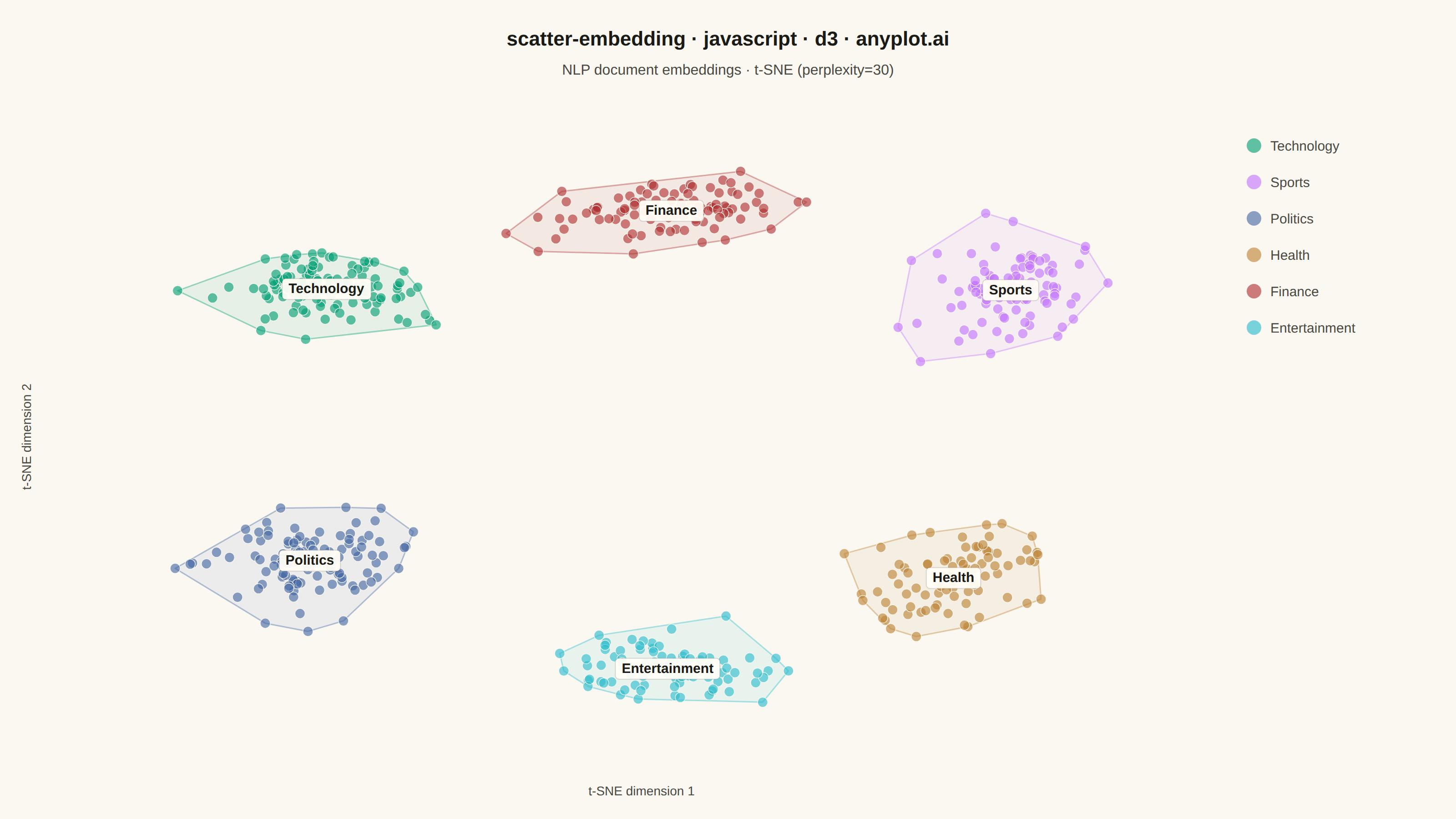
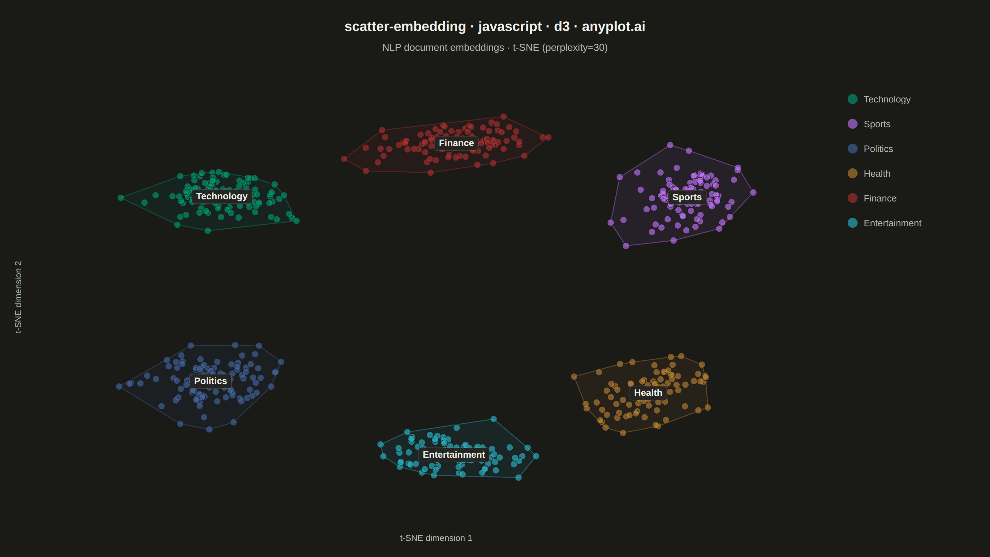
The same plot in 14 other libraries — JavaScript: Chart.js, Apache ECharts, Highcharts, MUI X Charts; Python: Altair, Bokeh, lets-plot, Matplotlib, Plotly, plotnine, Pygal, Seaborn; R: ggplot2; Julia: Makie.jl. Compare all 15 side by side: t-SNE and UMAP Embedding Visualization in Python, R, Julia and JavaScript.
A scatter plot displaying high-dimensional data projected into 2D space using non-linear dimensionality reduction techniques such as t-SNE or UMAP. Points are colored by cluster or class label, revealing groupings and latent structure in the data. This is a standard visualization in machine learning for exploring embeddings, single-cell RNA-seq data, and NLP document clustering, helping practitioners verify that learned representations capture meaningful distinctions.
// anyplot.ai
// scatter-embedding: t-SNE and UMAP Embedding Visualization
// Library: d3 7.9.0 | JavaScript 22.23.1
// Quality: 93/100 | Created: 2026-08-11

const t = window.ANYPLOT_TOKENS;
const { width, height } = window.ANYPLOT_SIZE;
const margin = { top: 130, right: 280, bottom: 70, left: 90 };
const iw = width - margin.left - margin.right;
const ih = height - margin.top - margin.bottom;

// --- Deterministic RNG (LCG + Box-Muller) -----------------------------------
let seed = 42;
const rand = () => {
  seed = (seed * 1103515245 + 12345) & 0x7fffffff;
  return seed / 0x7fffffff;
};
const randNormal = () => {
  const u1 = Math.max(rand(), 1e-6);
  const u2 = rand();
  return Math.sqrt(-2 * Math.log(u1)) * Math.cos(2 * Math.PI * u2);
};

// --- Data: synthetic NLP document embeddings, projected via t-SNE ----------
// Each topic cluster gets its own center, elongation, and rotation so the
// blobs read like genuine t-SNE output rather than perfect circles.
// Centers pushed further from the origin (vs. a tighter first draft) and the
// Technology/Finance ellipses de-aligned + slimmed so their spreads no longer
// bleed into one another near the top of the ring.
const clusterDefs = [
  { name: "Technology", n: 120, cx: -9.1, cy: 7.7, sx: 1.3, sy: 0.9, angle: -0.15 },
  { name: "Sports", n: 95, cx: 9.1, cy: 7.7, sx: 1.1, sy: 1.4, angle: -0.3 },
  { name: "Politics", n: 110, cx: -9.8, cy: -6.3, sx: 1.3, sy: 1.1, angle: 0.9 },
  { name: "Health", n: 85, cx: 7.7, cy: -7, sx: 1.0, sy: 1.6, angle: -0.6 },
  { name: "Finance", n: 100, cx: 0, cy: 11.9, sx: 1.5, sy: 0.8, angle: 0.1 },
  { name: "Entertainment", n: 90, cx: 0, cy: -11.9, sx: 1.5, sy: 0.9, angle: -0.2 },
];

const points = [];
for (const c of clusterDefs) {
  for (let i = 0; i < c.n; i++) {
    const rx = randNormal() * c.sx;
    const ry = randNormal() * c.sy;
    const px = c.cx + rx * Math.cos(c.angle) - ry * Math.sin(c.angle);
    const py = c.cy + rx * Math.sin(c.angle) + ry * Math.cos(c.angle);
    points.push({ x: px, y: py, cluster: c.name });
  }
}

const clusters = clusterDefs.map((c) => {
  const pts = points.filter((p) => p.cluster === c.name);
  return {
    name: c.name,
    cx: d3.mean(pts, (p) => p.x),
    cy: d3.mean(pts, (p) => p.y),
  };
});

// --- Scales -------------------------------------------------------------
const xExtent = d3.extent(points, (p) => p.x);
const yExtent = d3.extent(points, (p) => p.y);
const xPad = (xExtent[1] - xExtent[0]) * 0.1;
const yPad = (yExtent[1] - yExtent[0]) * 0.1;

const x = d3.scaleLinear().domain([xExtent[0] - xPad, xExtent[1] + xPad]).range([0, iw]);
const y = d3.scaleLinear().domain([yExtent[0] - yPad, yExtent[1] + yPad]).range([ih, 0]);
const color = d3.scaleOrdinal().domain(clusterDefs.map((c) => c.name)).range(t.palette);

// --- SVG mount ------------------------------------------------------------
const svg = d3.select("#container").append("svg").attr("width", width).attr("height", height);
const g = svg.append("g").attr("transform", `translate(${margin.left},${margin.top})`);

// --- Cluster hull outlines (d3.polygonHull) --------------------------------
// A genuine D3-distinctive technique: trace each cluster's convex hull in
// pixel space to give the grouping a deliberate visual boundary/focal shape
// beyond color alone, drawn beneath the points so markers stay on top.
const hullG = g.append("g").attr("class", "hulls");
for (const c of clusterDefs) {
  const hull = d3.polygonHull(
    points.filter((p) => p.cluster === c.name).map((p) => [x(p.x), y(p.y)])
  );
  if (!hull) continue;
  hullG
    .append("path")
    .attr("d", `M${hull.map((p) => p.join(",")).join("L")}Z`)
    .attr("fill", color(c.name))
    .attr("fill-opacity", 0.08)
    .attr("stroke", color(c.name))
    .attr("stroke-opacity", 0.4)
    .attr("stroke-width", 1.5)
    .attr("stroke-linejoin", "round");
}

// --- Points (moderate size + alpha to handle overlap at n=600) -------------
g.selectAll("circle")
  .data(points)
  .join("circle")
  .attr("cx", (d) => x(d.x))
  .attr("cy", (d) => y(d.y))
  .attr("r", 5.5)
  .attr("fill", (d) => color(d.cluster))
  .attr("fill-opacity", 0.62)
  .attr("stroke", t.pageBg)
  .attr("stroke-width", 0.6);

// --- Centroid labels (cluster name over a soft halo for legibility) --------
const centroidG = g
  .selectAll(".centroid")
  .data(clusters)
  .join("g")
  .attr("class", "centroid")
  .attr("transform", (d) => `translate(${x(d.cx)},${y(d.cy)})`);

centroidG.each(function (d) {
  const node = d3.select(this);
  const label = node
    .append("text")
    .attr("text-anchor", "middle")
    .attr("dy", "0.35em")
    .style("font-size", "15px")
    .style("font-weight", "600")
    .attr("fill", t.ink)
    .text(d.name);
  const bbox = label.node().getBBox();
  node
    .insert("rect", "text")
    .attr("x", bbox.x - 7)
    .attr("y", bbox.y - 3)
    .attr("width", bbox.width + 14)
    .attr("height", bbox.height + 6)
    .attr("rx", 4)
    .attr("fill", t.elevatedBg)
    .attr("fill-opacity", 0.95)
    .attr("stroke", t.grid)
    .attr("stroke-width", 1);
});

// --- Axis labels (no tick labels — embedding coordinates are not directly
// interpretable, only relative position and clustering carry meaning) ------
g.append("text")
  .attr("x", iw / 2)
  .attr("y", ih + 44)
  .attr("text-anchor", "middle")
  .attr("fill", t.inkSoft)
  .style("font-size", "14px")
  .text("t-SNE dimension 1");

g.append("text")
  .attr("transform", `translate(${-56},${ih / 2}) rotate(-90)`)
  .attr("text-anchor", "middle")
  .attr("fill", t.inkSoft)
  .style("font-size", "14px")
  .text("t-SNE dimension 2");

// --- Legend -----------------------------------------------------------------
const legend = svg
  .append("g")
  .attr("transform", `translate(${margin.left + iw + 50},${margin.top + 30})`);

const legendItems = legend
  .selectAll(".legend-item")
  .data(clusterDefs)
  .join("g")
  .attr("class", "legend-item")
  .attr("transform", (d, i) => `translate(0,${i * 40})`);

legendItems
  .append("circle")
  .attr("r", 8)
  .attr("cx", 8)
  .attr("cy", 0)
  .attr("fill", (d) => color(d.name))
  .attr("fill-opacity", 0.62);

legendItems
  .append("text")
  .attr("x", 26)
  .attr("y", 0)
  .attr("dy", "0.35em")
  .attr("fill", t.inkSoft)
  .style("font-size", "15px")
  .text((d) => d.name);

// --- Title + subtitle --------------------------------------------------------
svg
  .append("text")
  .attr("x", width / 2)
  .attr("y", 50)
  .attr("text-anchor", "middle")
  .attr("fill", t.ink)
  .style("font-size", "22px")
  .style("font-weight", "600")
  .text("scatter-embedding · javascript · d3 · anyplot.ai");

svg
  .append("text")
  .attr("x", width / 2)
  .attr("y", 82)
  .attr("text-anchor", "middle")
  .attr("fill", t.inkSoft)
  .style("font-size", "16px")
  .text("NLP document embeddings · t-SNE (perplexity=30)");
Runnable source as JSON, for any HTTP client: https://api.anyplot.ai/specs/scatter-embedding/d3/code. Any spec id and library id listed in llms-full.txt fit the same URL shape; every URL below is complete and callable.
{
  "spec_id": "scatter-embedding",
  "language": "javascript",
  "library": "d3",
  "page": "https://anyplot.ai/scatter-embedding/javascript/d3",
  "hub": "https://anyplot.ai/scatter-embedding",
  "code_json": "https://api.anyplot.ai/specs/scatter-embedding/d3/code",
  "spec_json": "https://api.anyplot.ai/specs/scatter-embedding",
  "render_light_png": "https://storage.googleapis.com/anyplot-images/plots/scatter-embedding/javascript/d3/plot-light.png",
  "render_dark_png": "https://storage.googleapis.com/anyplot-images/plots/scatter-embedding/javascript/d3/plot-dark.png",
  "interactive_light_html": "https://storage.googleapis.com/anyplot-images/plots/scatter-embedding/javascript/d3/plot-light.html",
  "interactive_dark_html": "https://storage.googleapis.com/anyplot-images/plots/scatter-embedding/javascript/d3/plot-dark.html",
  "quality_score": 93.0,
  "license": "MIT",
  "guide": "https://anyplot.ai/llms.txt"
}
Part of t-SNE and UMAP Embedding Visualization on anyplot.ai.