The same plot in 14 other libraries — Python: Altair, lets-plot, Matplotlib, Plotly, plotnine, Pygal, Seaborn; R: ggplot2; Julia: Makie.jl; JavaScript: Chart.js, D3.js, Apache ECharts, Highcharts, MUI X Charts. Compare all 15 side by side: t-SNE and UMAP Embedding Visualization in Python, R, Julia and JavaScript.
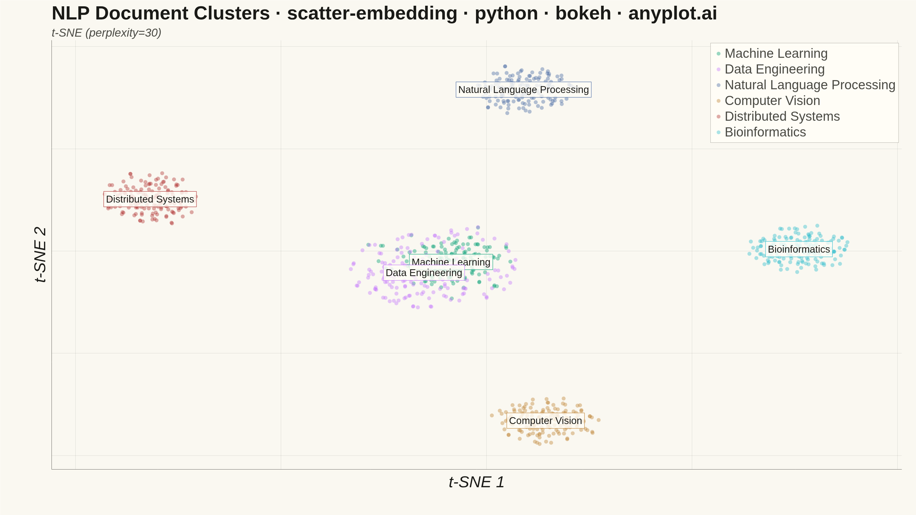
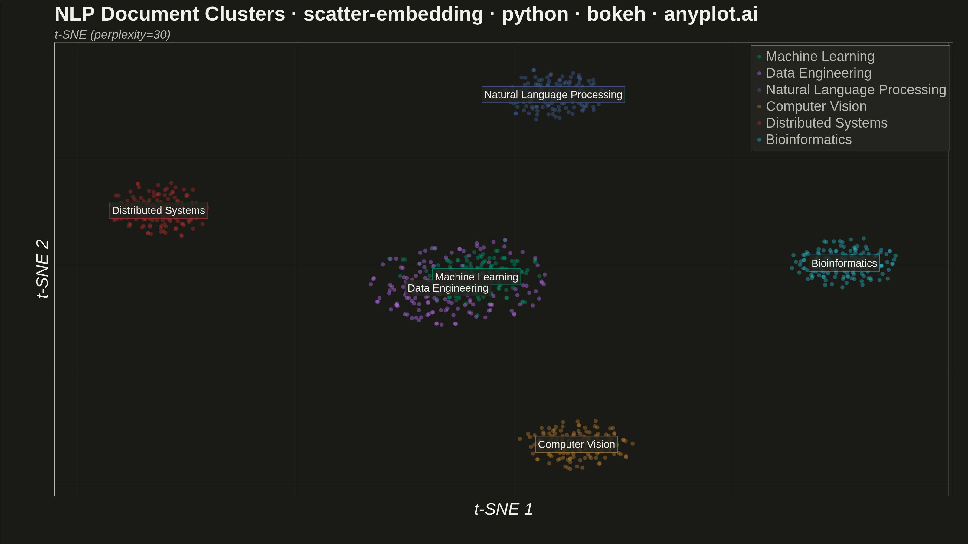
A scatter plot displaying high-dimensional data projected into 2D space using non-linear dimensionality reduction techniques such as t-SNE or UMAP. Points are colored by cluster or class label, revealing groupings and latent structure in the data. This is a standard visualization in machine learning for exploring embeddings, single-cell RNA-seq data, and NLP document clustering, helping practitioners verify that learned representations capture meaningful distinctions.
""" anyplot.ai
scatter-embedding: t-SNE and UMAP Embedding Visualization
Library: bokeh 3.9.2 | Python 3.13.14
Quality: 91/100 | Updated: 2026-08-11
"""

import os
import sys
import time
from pathlib import Path


sys.path = [p for p in sys.path if "implementations" not in p]

import numpy as np
from bokeh.io import output_file, save
from bokeh.models import ColumnDataSource, Label, Range1d, Title
from bokeh.plotting import figure
from selenium import webdriver
from selenium.webdriver.chrome.options import Options
from sklearn.datasets import make_blobs
from sklearn.manifold import TSNE


# Theme tokens
THEME = os.getenv("ANYPLOT_THEME", "light")
PAGE_BG = "#FAF8F1" if THEME == "light" else "#1A1A17"
ELEVATED_BG = "#FFFDF6" if THEME == "light" else "#242420"
INK = "#1A1A17" if THEME == "light" else "#F0EFE8"
INK_SOFT = "#4A4A44" if THEME == "light" else "#B8B7B0"

# Imprint palette — canonical categorical order, first series always brand green
IMPRINT = ["#009E73", "#C475FD", "#4467A3", "#BD8233", "#AE3030", "#2ABCCD"]
CLUSTER_NAMES = [
    "Machine Learning",
    "Data Engineering",
    "Natural Language Processing",
    "Computer Vision",
    "Distributed Systems",
    "Bioinformatics",
]

# Data — synthetic high-dimensional document embeddings reduced via t-SNE.
# Cluster centers and spreads are varied (rather than uniform) to mimic the
# ambiguity real embeddings show: Data Engineering is nudged close to Machine
# Learning so the two overlap slightly, and cluster_std differs per group.
np.random.seed(42)
n_features = 20
centers = np.random.uniform(-10, 10, size=(6, n_features))
centers[1] = centers[0] + np.random.normal(scale=1.5, size=n_features)
cluster_std = [2.5, 3.2, 2.1, 2.9, 1.9, 3.5]
X, labels = make_blobs(n_samples=900, n_features=n_features, centers=centers, cluster_std=cluster_std)
tsne = TSNE(n_components=2, perplexity=30, random_state=42, max_iter=1000)
embedding = tsne.fit_transform(X)

# Fit axes to the 2nd-98th percentile of the data rather than the raw min/max —
# a handful of t-SNE stragglers otherwise inflate the range and leave large
# empty margins on one side of the canvas (VQ-05 in the previous review).
x_lo, x_hi = np.percentile(embedding[:, 0], [2, 98])
y_lo, y_hi = np.percentile(embedding[:, 1], [2, 98])
x_pad = (x_hi - x_lo) * 0.10
y_pad = (y_hi - y_lo) * 0.10

# Plot — canonical 3200x1800 landscape canvas (Step 0 contract)
W, H = 3200, 1800
p = figure(
    width=W,
    height=H,
    title="NLP Document Clusters · scatter-embedding · python · bokeh · anyplot.ai",
    x_range=Range1d(x_lo - x_pad, x_hi + x_pad),
    y_range=Range1d(y_lo - y_pad, y_hi + y_pad),
    tools="pan,wheel_zoom,box_zoom,reset,hover",
    tooltips=[("Cluster", "@cluster")],
    toolbar_location=None,  # default toolbar shrinks the saved PNG below `height=`
    min_border_bottom=160,
    min_border_left=180,
    min_border_top=140,  # extra room for the two-line title + subtitle stack
    min_border_right=50,
)

p.add_layout(
    Title(text="t-SNE (perplexity=30)", text_font_size="30pt", text_color=INK_SOFT, text_font_style="italic"), "above"
)

# Chrome
p.background_fill_color = PAGE_BG
p.border_fill_color = PAGE_BG
p.outline_line_color = None

p.title.text_color = INK
p.title.text_font_size = "50pt"
p.title.text_font_style = "bold"

p.xaxis.axis_label = "t-SNE 1"
p.yaxis.axis_label = "t-SNE 2"
p.xaxis.axis_label_text_color = INK
p.yaxis.axis_label_text_color = INK
p.xaxis.axis_label_text_font_size = "42pt"
p.yaxis.axis_label_text_font_size = "42pt"

# Hide tick labels — embedding coordinates are not directly interpretable
p.xaxis.major_label_text_alpha = 0
p.yaxis.major_label_text_alpha = 0
p.xaxis.major_tick_line_alpha = 0
p.yaxis.major_tick_line_alpha = 0
p.xaxis.minor_tick_line_alpha = 0
p.yaxis.minor_tick_line_alpha = 0

p.xaxis.axis_line_color = INK_SOFT
p.yaxis.axis_line_color = INK_SOFT

p.xgrid.grid_line_color = INK
p.ygrid.grid_line_color = INK
p.xgrid.grid_line_alpha = 0.15
p.ygrid.grid_line_alpha = 0.15

# One scatter call per cluster so Bokeh assigns legend entries
for i, (name, color) in enumerate(zip(CLUSTER_NAMES, IMPRINT, strict=False)):
    mask = labels == i
    source = ColumnDataSource(
        data={"x": embedding[mask, 0], "y": embedding[mask, 1], "cluster": [name] * int(mask.sum())}
    )
    p.scatter(
        x="x",
        y="y",
        source=source,
        color=color,
        size=14,
        alpha=0.40,
        line_color=PAGE_BG,
        line_width=0.6,
        legend_label=name,
    )

# Centroid annotations — label each cluster at its centre for storytelling
for i, (name, color) in enumerate(zip(CLUSTER_NAMES, IMPRINT, strict=False)):
    mask = labels == i
    cx = float(embedding[mask, 0].mean())
    cy = float(embedding[mask, 1].mean())
    centroid_label = Label(
        x=cx,
        y=cy,
        text=name,
        text_font_size="26pt",
        text_color=INK,
        text_align="center",
        text_baseline="middle",
        background_fill_color=ELEVATED_BG,
        background_fill_alpha=0.80,
        border_line_color=color,
        border_line_width=2,
        border_line_alpha=0.7,
        padding=8,
    )
    p.add_layout(centroid_label)

# Style legend
p.legend.background_fill_color = ELEVATED_BG
p.legend.border_line_color = INK_SOFT
p.legend.label_text_color = INK_SOFT
p.legend.label_text_font_size = "34pt"
p.legend.glyph_height = 34
p.legend.glyph_width = 34
p.legend.location = "top_right"
p.legend.click_policy = "hide"

# Save HTML
output_file(f"plot-{THEME}.html")
save(p)

# Screenshot via headless Chrome
opts = Options()
for arg in (
    "--headless=new",
    "--no-sandbox",
    "--disable-dev-shm-usage",
    "--disable-gpu",
    f"--window-size={W},{H}",
    "--hide-scrollbars",
):
    opts.add_argument(arg)
driver = webdriver.Chrome(options=opts)
driver.set_window_size(W, H)
driver.get(f"file://{Path(f'plot-{THEME}.html').resolve()}")
# Headless Chrome's --window-size sets the OUTER window, which still reserves a
# phantom title-bar height even headless — pin the viewport exactly via CDP.
driver.execute_cdp_cmd(
    "Emulation.setDeviceMetricsOverride", {"width": W, "height": H, "deviceScaleFactor": 1, "mobile": False}
)
time.sleep(3)
driver.save_screenshot(f"plot-{THEME}.png")
driver.quit()
Runnable source as JSON, for any HTTP client: https://api.anyplot.ai/specs/scatter-embedding/bokeh/code. Any spec id and library id listed in llms-full.txt fit the same URL shape; every URL below is complete and callable.
{
  "spec_id": "scatter-embedding",
  "language": "python",
  "library": "bokeh",
  "page": "https://anyplot.ai/scatter-embedding/python/bokeh",
  "hub": "https://anyplot.ai/scatter-embedding",
  "code_json": "https://api.anyplot.ai/specs/scatter-embedding/bokeh/code",
  "spec_json": "https://api.anyplot.ai/specs/scatter-embedding",
  "render_light_png": "https://storage.googleapis.com/anyplot-images/plots/scatter-embedding/python/bokeh/plot-light.png",
  "render_dark_png": "https://storage.googleapis.com/anyplot-images/plots/scatter-embedding/python/bokeh/plot-dark.png",
  "interactive_light_html": "https://storage.googleapis.com/anyplot-images/plots/scatter-embedding/python/bokeh/plot-light.html",
  "interactive_dark_html": "https://storage.googleapis.com/anyplot-images/plots/scatter-embedding/python/bokeh/plot-dark.html",
  "quality_score": 91.0,
  "license": "MIT",
  "guide": "https://anyplot.ai/llms.txt"
}
Part of t-SNE and UMAP Embedding Visualization on anyplot.ai.