The same plot in 14 other libraries — Python: Altair, Bokeh, lets-plot, Matplotlib, Plotly, plotnine, Pygal, Seaborn; R: ggplot2; JavaScript: Chart.js, D3.js, Apache ECharts, Highcharts, MUI X Charts. Compare all 15 side by side: t-SNE and UMAP Embedding Visualization in Python, R, Julia and JavaScript.
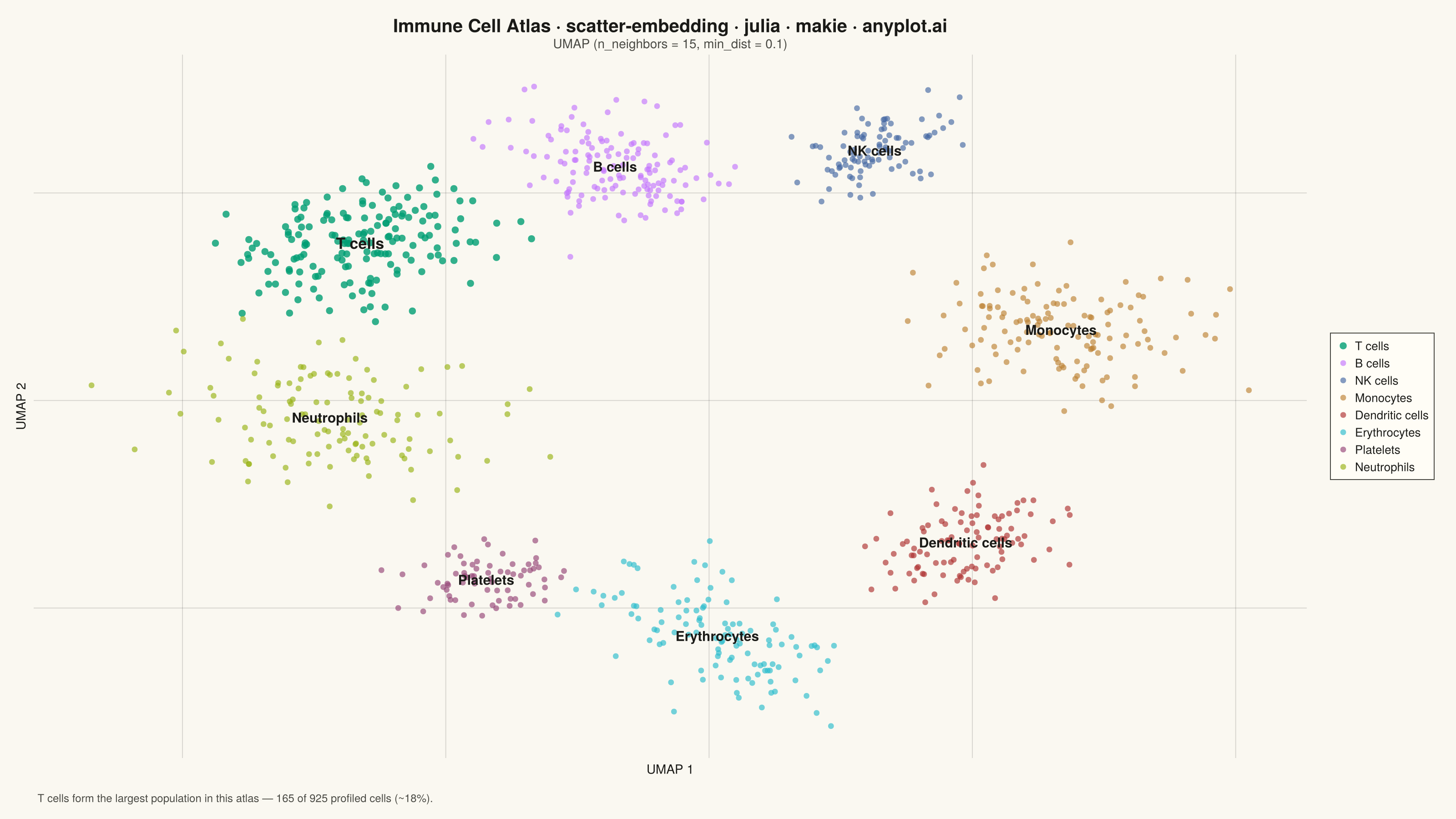
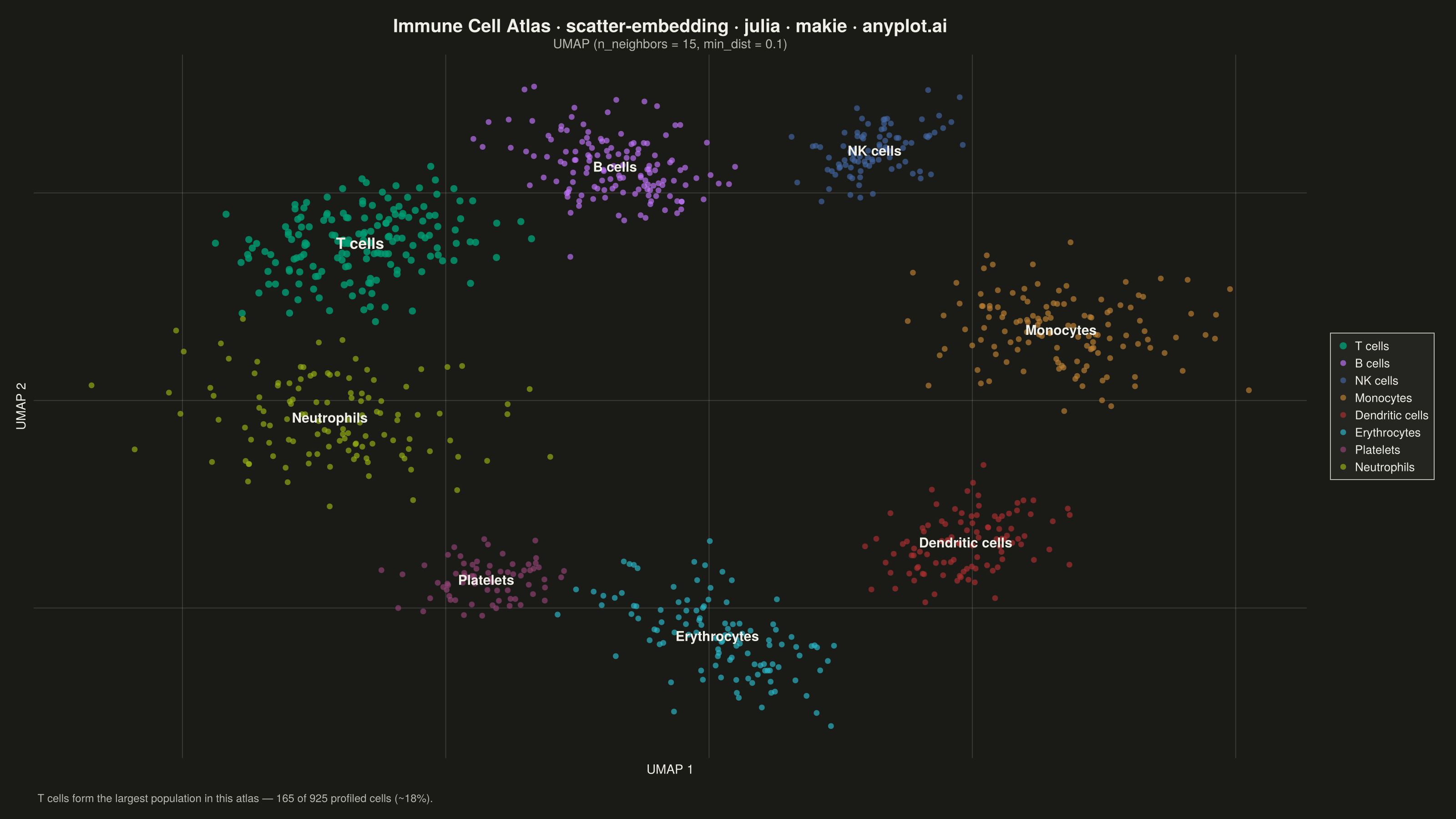
A scatter plot displaying high-dimensional data projected into 2D space using non-linear dimensionality reduction techniques such as t-SNE or UMAP. Points are colored by cluster or class label, revealing groupings and latent structure in the data. This is a standard visualization in machine learning for exploring embeddings, single-cell RNA-seq data, and NLP document clustering, helping practitioners verify that learned representations capture meaningful distinctions.
# anyplot.ai
# scatter-embedding: t-SNE and UMAP Embedding Visualization
# Library: makie 0.21.9 | Julia 1.11.9
# Quality: 94/100 | Created: 2026-08-11

using CairoMakie
using Colors
using Random
using Statistics

Random.seed!(42)

# Theme tokens
const THEME       = get(ENV, "ANYPLOT_THEME", "light")
const PAGE_BG     = THEME == "light" ? colorant"#FAF8F1" : colorant"#1A1A17"
const ELEVATED_BG = THEME == "light" ? colorant"#FFFDF6" : colorant"#242420"
const INK         = THEME == "light" ? colorant"#1A1A17" : colorant"#F0EFE8"
const INK_SOFT    = THEME == "light" ? colorant"#4A4A44" : colorant"#B8B7B0"

const IMPRINT_PALETTE = [
    colorant"#009E73",  # 1 — brand green (first series)
    colorant"#C475FD",  # 2 — lavender
    colorant"#4467A3",  # 3 — blue
    colorant"#BD8233",  # 4 — ochre
    colorant"#AE3030",  # 5 — matte red
    colorant"#2ABCCD",  # 6 — cyan
    colorant"#954477",  # 7 — rose
    colorant"#99B314",  # 8 — lime
]

# Data — synthetic UMAP projection of a single-cell RNA-seq immune atlas,
# 8 organic (anisotropic, unequal-density) clusters mimicking real embeddings
cell_types = ["T cells", "B cells", "NK cells", "Monocytes",
              "Dendritic cells", "Erythrocytes", "Platelets", "Neutrophils"]
n_clusters = length(cell_types)

centers = [(-6.5, 3.8), (-1.8, 5.6), (3.2, 6.0), (6.6, 1.8),
           (4.8, -3.4), (0.2, -5.6), (-4.2, -4.4), (-7.2, -0.6)]
spreads  = [1.3, 1.1, 0.9, 1.4, 1.0, 1.2, 0.75, 1.5]
rotation = [0.3, -0.4, 0.6, -0.2, 0.5, -0.6, 0.2, -0.3]
sizes    = [165, 140, 90, 130, 100, 110, 70, 120]  # 500-5000 pt range, high density

xs = Float64[]
ys = Float64[]
group_idx = Int[]
for i in 1:n_clusters
    cx, cy = centers[i]
    s = spreads[i]
    θ = rotation[i]
    dx = s .* randn(sizes[i])
    dy = 0.6s .* randn(sizes[i])
    append!(xs, cx .+ dx .* cos(θ) .- dy .* sin(θ))
    append!(ys, cy .+ dx .* sin(θ) .+ dy .* cos(θ))
    append!(group_idx, fill(i, sizes[i]))
end

# --- Figure ------------------------------------------------------------------
fig = Figure(
    size            = (1600, 900),
    fontsize        = 14,
    backgroundcolor = PAGE_BG,
)

ax = Axis(
    fig[1, 1];
    title              = "Immune Cell Atlas · scatter-embedding · julia · makie · anyplot.ai",
    titlesize          = 20,
    titlecolor         = INK,
    subtitle           = "UMAP (n_neighbors = 15, min_dist = 0.1)",
    subtitlesize       = 14,
    subtitlecolor      = INK_SOFT,
    xlabel             = "UMAP 1",
    ylabel             = "UMAP 2",
    xlabelsize         = 14,
    ylabelsize         = 14,
    xlabelcolor        = INK,
    ylabelcolor        = INK,
    xticklabelsvisible = false,
    yticklabelsvisible = false,
    xticksvisible      = false,
    yticksvisible      = false,
    backgroundcolor    = PAGE_BG,
    xgridcolor         = RGBAf(INK.r, INK.g, INK.b, 0.15f0),
    ygridcolor         = RGBAf(INK.r, INK.g, INK.b, 0.15f0),
    xminorgridvisible  = false,
    yminorgridvisible  = false,
)

# Embedding coordinates carry no meaningful axis position, so drop the frame
# entirely (style guide's "minimal scatter" spine alternative) rather than
# keeping the default L-shape around hidden ticks.
hidespines!(ax)

# --- Points, one scatter! call per cluster for a clean discrete legend -------
# T cells is the largest population (165 of 925 cells, ~18%); a modest bump
# in marker size/opacity gives it visual priority over the other 7 clusters.
largest = argmax(sizes)
for i in 1:n_clusters
    mask = group_idx .== i
    emphasized = i == largest
    scatter!(ax, xs[mask], ys[mask];
        color       = (IMPRINT_PALETTE[i], emphasized ? 0.8 : 0.65),
        markersize  = emphasized ? 11 : 9,
        strokewidth = 0,
        label       = cell_types[i],
    )
end

# --- Centroid labels — direct per-cluster labeling. 8 series exceeds safe
# --- color-only discrimination, so labels add a redundant, non-color cue. ---
for i in 1:n_clusters
    cx, cy = mean(xs[group_idx .== i]), mean(ys[group_idx .== i])
    text!(ax, cx, cy;
        text     = cell_types[i],
        color    = INK,
        fontsize = i == largest ? 17 : 15,
        font     = :bold,
        align    = (:center, :center),
    )
end

# --- Legend ------------------------------------------------------------------
Legend(
    fig[1, 2],
    ax,
    framecolor      = INK_SOFT,
    backgroundcolor = ELEVATED_BG,
    labelcolor      = INK,
    labelsize       = 13,
    patchsize       = (16, 16),
    margin          = (8, 8, 8, 8),
)

# --- Footnote — layout-level polish + the storytelling cue behind the -------
# --- T-cell emphasis above (Makie's grid layout takes a footnote row as ----
# --- naturally as a plot column). --------------------------------------------
Label(
    fig[2, 1:2],
    "T cells form the largest population in this atlas — 165 of 925 profiled cells (~18%).",
    fontsize  = 12,
    color     = INK_SOFT,
    halign    = :left,
    padding   = (4, 0, 0, 0),
)

# --- Save --------------------------------------------------------------------
save("plot-$(THEME).png", fig; px_per_unit = 2)
Runnable source as JSON, for any HTTP client: https://api.anyplot.ai/specs/scatter-embedding/makie/code. Any spec id and library id listed in llms-full.txt fit the same URL shape; every URL below is complete and callable.
{
  "spec_id": "scatter-embedding",
  "language": "julia",
  "library": "makie",
  "page": "https://anyplot.ai/scatter-embedding/julia/makie",
  "hub": "https://anyplot.ai/scatter-embedding",
  "code_json": "https://api.anyplot.ai/specs/scatter-embedding/makie/code",
  "spec_json": "https://api.anyplot.ai/specs/scatter-embedding",
  "render_light_png": "https://storage.googleapis.com/anyplot-images/plots/scatter-embedding/julia/makie/plot-light.png",
  "render_dark_png": "https://storage.googleapis.com/anyplot-images/plots/scatter-embedding/julia/makie/plot-dark.png",
  "quality_score": 94.0,
  "license": "MIT",
  "guide": "https://anyplot.ai/llms.txt"
}
Part of t-SNE and UMAP Embedding Visualization on anyplot.ai.