The same plot in 14 other libraries — Python: Altair, Bokeh, lets-plot, Matplotlib, plotnine, Pygal, Seaborn; R: ggplot2; Julia: Makie.jl; JavaScript: Chart.js, D3.js, Apache ECharts, Highcharts, MUI X Charts. Compare all 15 side by side: t-SNE and UMAP Embedding Visualization in Python, R, Julia and JavaScript.
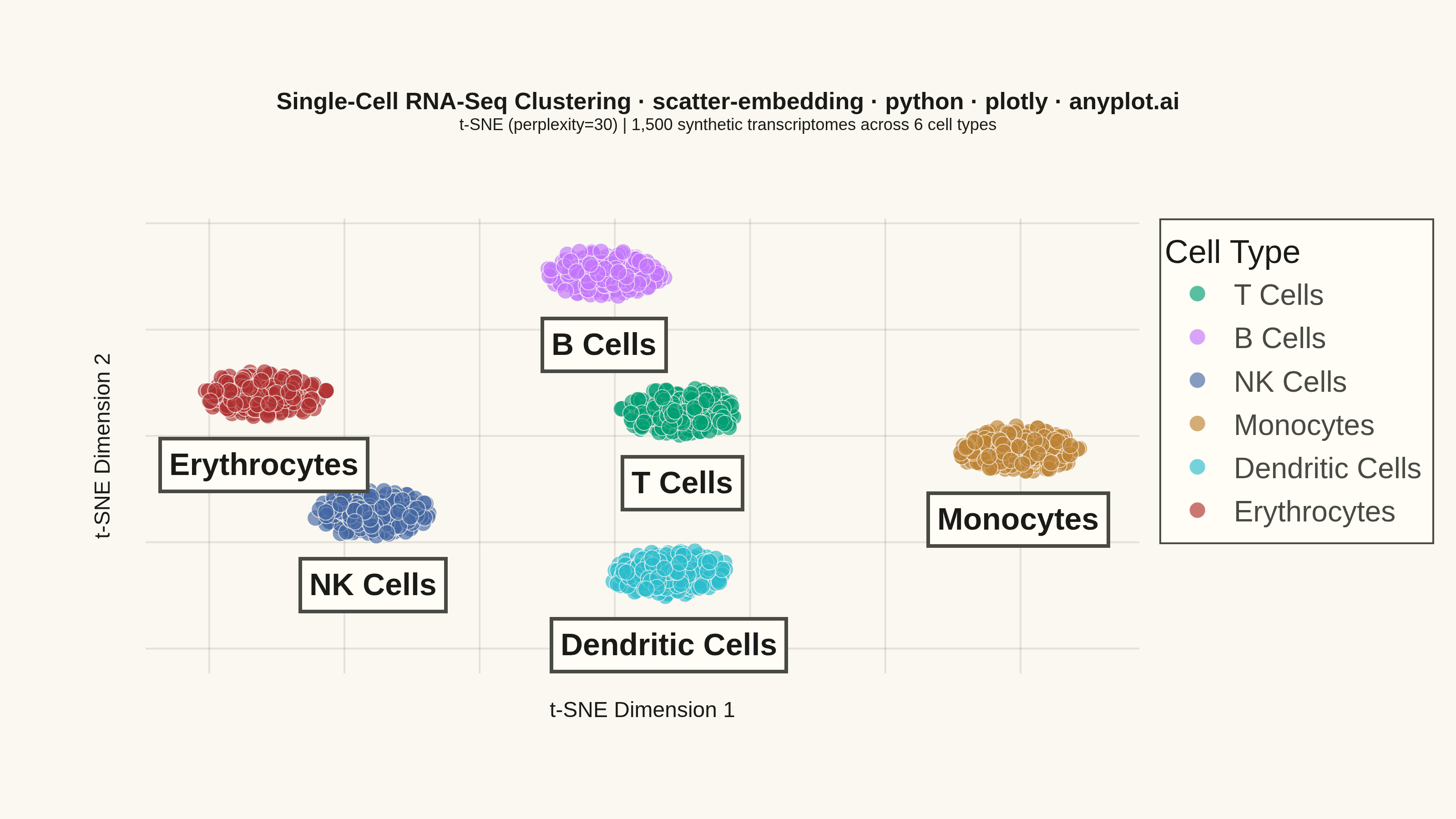
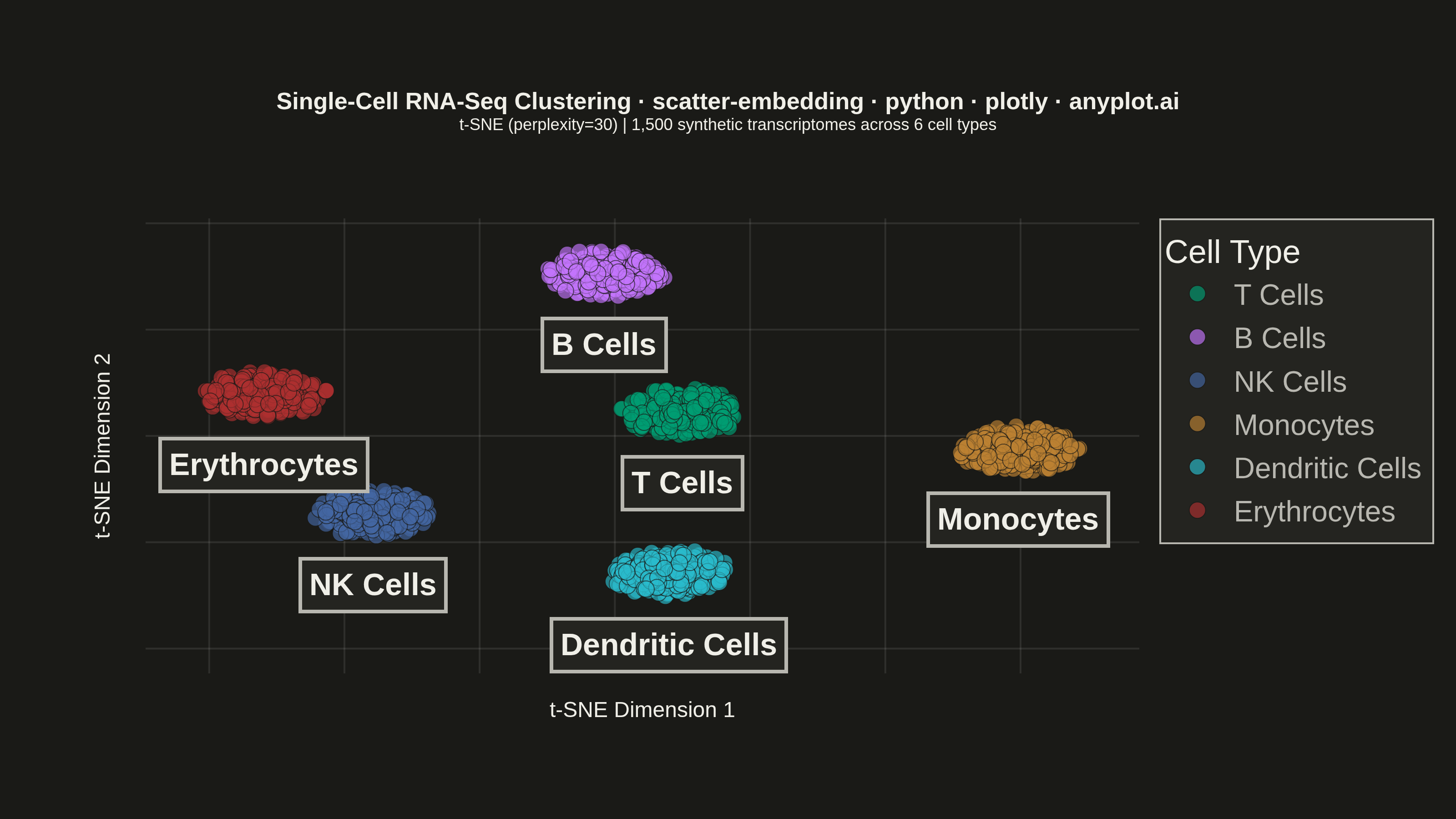
A scatter plot displaying high-dimensional data projected into 2D space using non-linear dimensionality reduction techniques such as t-SNE or UMAP. Points are colored by cluster or class label, revealing groupings and latent structure in the data. This is a standard visualization in machine learning for exploring embeddings, single-cell RNA-seq data, and NLP document clustering, helping practitioners verify that learned representations capture meaningful distinctions.
""" anyplot.ai
scatter-embedding: t-SNE and UMAP Embedding Visualization
Library: plotly 6.9.0 | Python 3.13.14
Quality: 87/100 | Updated: 2026-08-11
"""

import os

import numpy as np
import plotly.graph_objects as go
from sklearn.datasets import make_blobs
from sklearn.manifold import TSNE


# Theme tokens
THEME = os.getenv("ANYPLOT_THEME", "light")
PAGE_BG = "#FAF8F1" if THEME == "light" else "#1A1A17"
ELEVATED_BG = "#FFFDF6" if THEME == "light" else "#242420"
INK = "#1A1A17" if THEME == "light" else "#F0EFE8"
INK_SOFT = "#4A4A44" if THEME == "light" else "#B8B7B0"
GRID = "rgba(26,26,23,0.10)" if THEME == "light" else "rgba(240,239,232,0.10)"

# Imprint palette in canonical order, except Erythrocytes takes the matte-red
# anchor (#AE3030) for its blood association (default-style-guide.md "Semantic
# exception") instead of its ordinal position 6.
CELL_TYPES = ["T Cells", "B Cells", "NK Cells", "Monocytes", "Dendritic Cells", "Erythrocytes"]
IMPRINT = ["#009E73", "#C475FD", "#4467A3", "#BD8233", "#2ABCCD", "#AE3030"]

# Data — simulate single-cell RNA-seq transcriptomes across 50 marker genes
np.random.seed(42)

n_clusters = len(CELL_TYPES)
gene_expression, labels = make_blobs(
    n_samples=1500, n_features=50, centers=n_clusters, cluster_std=6.0, center_box=(-30, 30), random_state=42
)

# Reduce to 2D with t-SNE
tsne = TSNE(n_components=2, perplexity=30, random_state=42, max_iter=1000)
embedding_2d = tsne.fit_transform(gene_expression)

# Plot — one trace per cell type
fig = go.Figure()

for i, cell_type in enumerate(CELL_TYPES):
    mask = labels == i
    fig.add_trace(
        go.Scatter(
            x=embedding_2d[mask, 0],
            y=embedding_2d[mask, 1],
            mode="markers",
            name=cell_type,
            marker={"color": IMPRINT[i], "size": 9, "opacity": 0.65, "line": {"color": PAGE_BG, "width": 0.5}},
            hovertemplate="<b>%{fullData.name}</b><br>t-SNE 1: %{x:.2f}<br>t-SNE 2: %{y:.2f}<extra></extra>",
        )
    )

# Annotate cluster centroids — offset below each cluster's point cloud so the
# label box sits beneath the markers instead of covering them
y_margin = 0.06 * (embedding_2d[:, 1].max() - embedding_2d[:, 1].min())
for i, cell_type in enumerate(CELL_TYPES):
    mask = labels == i
    cx = float(embedding_2d[mask, 0].mean())
    cy_bottom = float(embedding_2d[mask, 1].min()) - y_margin
    fig.add_annotation(
        x=cx,
        y=cy_bottom,
        yanchor="top",
        text=f"<b>{cell_type}</b>",
        showarrow=False,
        font={"size": 17, "color": INK},
        bgcolor=ELEVATED_BG,
        bordercolor=INK_SOFT,
        borderwidth=2,
        borderpad=4,
        opacity=1.0,
    )

# Layout
title_text = "Single-Cell RNA-Seq Clustering · scatter-embedding · python · plotly · anyplot.ai"
fig.update_layout(
    autosize=False,
    width=800,
    height=450,
    title={
        "text": (
            f"<b>{title_text}</b>"
            "<br><sup>t-SNE (perplexity=30) | 1,500 synthetic transcriptomes across 6 cell types</sup>"
        ),
        "font": {"size": 13, "color": INK},
        "x": 0.5,
        "xanchor": "center",
    },
    paper_bgcolor=PAGE_BG,
    plot_bgcolor=PAGE_BG,
    font={"color": INK},
    xaxis={
        "title": {"text": "t-SNE Dimension 1", "font": {"size": 12, "color": INK}},
        "showticklabels": False,
        "showgrid": True,
        "gridcolor": GRID,
        "showline": False,
        "zeroline": False,
    },
    yaxis={
        "title": {"text": "t-SNE Dimension 2", "font": {"size": 12, "color": INK}},
        "showticklabels": False,
        "showgrid": True,
        "gridcolor": GRID,
        "showline": False,
        "zeroline": False,
    },
    legend={
        "bgcolor": ELEVATED_BG,
        "bordercolor": INK_SOFT,
        "borderwidth": 1,
        "font": {"size": 16, "color": INK_SOFT},
        "title": {"text": "Cell Type", "font": {"size": 18, "color": INK}},
    },
    hoverlabel={"bgcolor": ELEVATED_BG, "bordercolor": INK_SOFT, "font": {"color": INK, "size": 14}},
    margin={"l": 80, "r": 80, "t": 120, "b": 80},
)

# Save
fig.write_image(f"plot-{THEME}.png", width=800, height=450, scale=4)
fig.write_html(f"plot-{THEME}.html", include_plotlyjs="cdn")
Runnable source as JSON, for any HTTP client: https://api.anyplot.ai/specs/scatter-embedding/plotly/code. Any spec id and library id listed in llms-full.txt fit the same URL shape; every URL below is complete and callable.
{
  "spec_id": "scatter-embedding",
  "language": "python",
  "library": "plotly",
  "page": "https://anyplot.ai/scatter-embedding/python/plotly",
  "hub": "https://anyplot.ai/scatter-embedding",
  "code_json": "https://api.anyplot.ai/specs/scatter-embedding/plotly/code",
  "spec_json": "https://api.anyplot.ai/specs/scatter-embedding",
  "render_light_png": "https://storage.googleapis.com/anyplot-images/plots/scatter-embedding/python/plotly/plot-light.png",
  "render_dark_png": "https://storage.googleapis.com/anyplot-images/plots/scatter-embedding/python/plotly/plot-dark.png",
  "interactive_light_html": "https://storage.googleapis.com/anyplot-images/plots/scatter-embedding/python/plotly/plot-light.html",
  "interactive_dark_html": "https://storage.googleapis.com/anyplot-images/plots/scatter-embedding/python/plotly/plot-dark.html",
  "quality_score": 87.0,
  "license": "MIT",
  "guide": "https://anyplot.ai/llms.txt"
}
Part of t-SNE and UMAP Embedding Visualization on anyplot.ai.