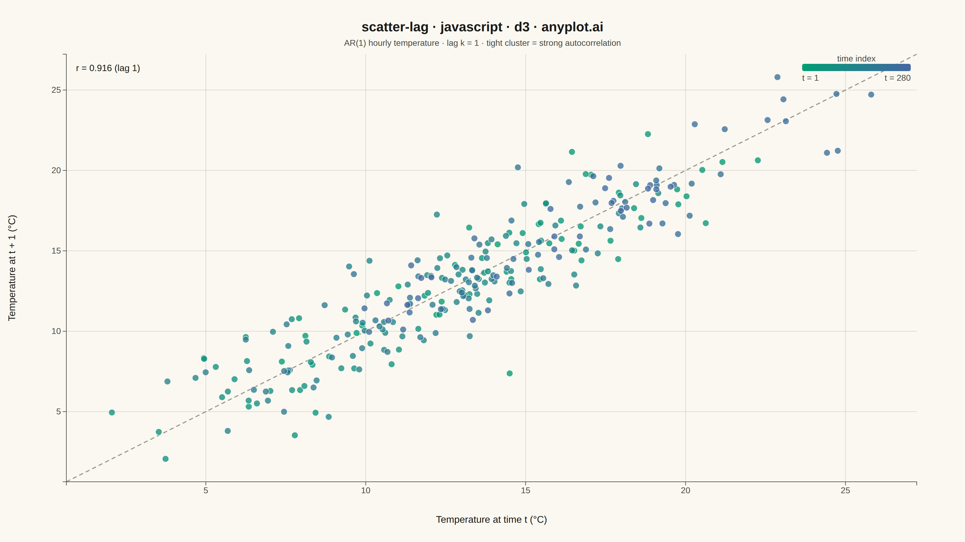
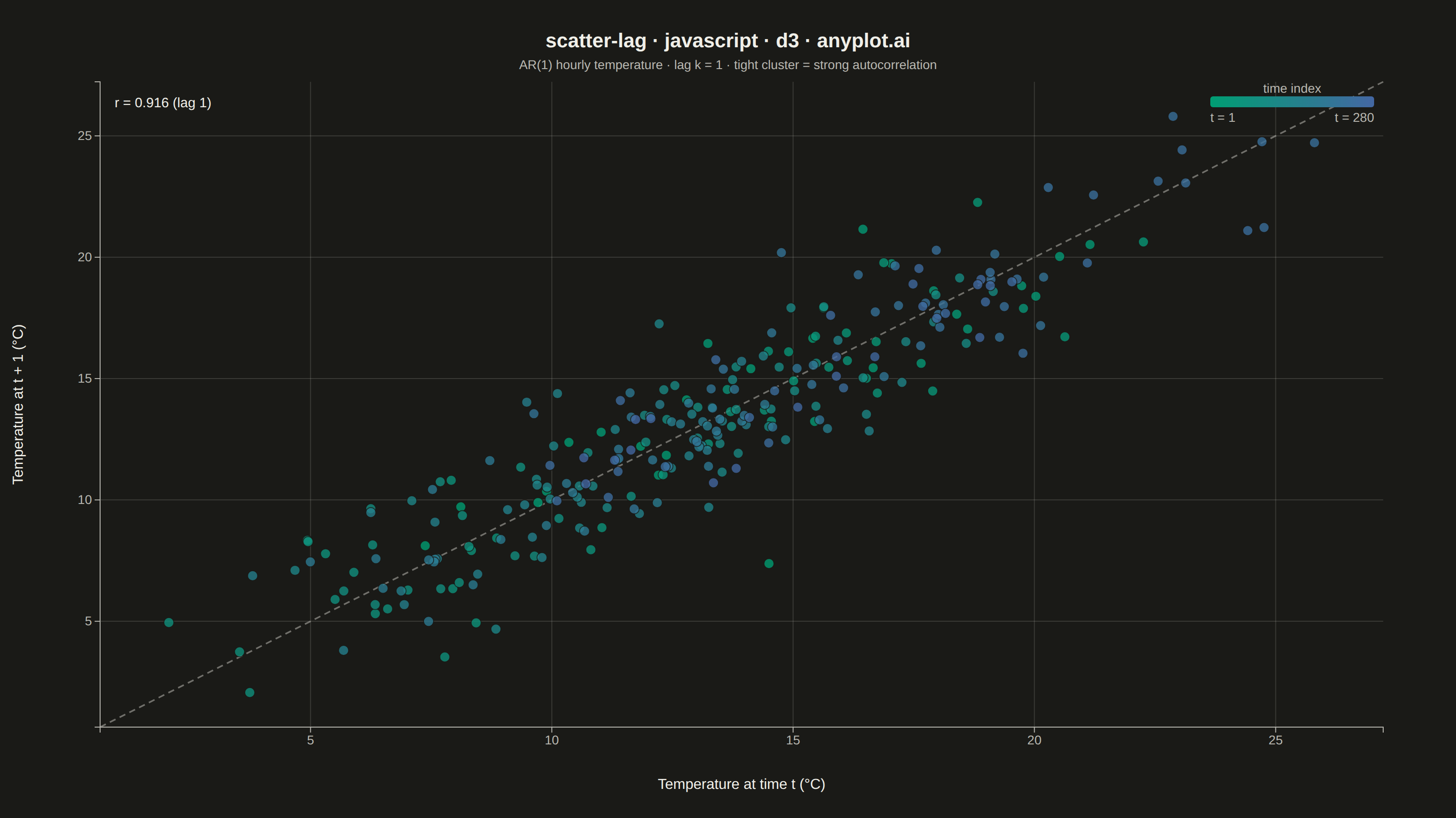
The same plot in 14 other libraries — JavaScript: Chart.js, Apache ECharts, Highcharts, MUI X Charts; Python: Altair, Bokeh, lets-plot, Matplotlib, Plotly, plotnine, Pygal, Seaborn; R: ggplot2; Julia: Makie.jl. Compare all 15 side by side: Lag Plot for Time Series Autocorrelation Diagnosis in Python, R, Julia and JavaScript.
A lag plot is a scatter plot of a time series against a lagged version of itself, plotting y(t) on the x-axis versus y(t+k) on the y-axis for a given lag order k. If the data is purely random, points scatter uniformly with no visible structure; if autocorrelation is present, distinctive patterns emerge — linear clusters for autoregressive processes, elliptical shapes for seasonal data. This provides a quick visual diagnostic for time series dependence, complementing numerical tools like ACF/PACF.
// anyplot.ai
// scatter-lag: Lag Plot for Time Series Autocorrelation Diagnosis
// Library: d3 7.9.0 | JavaScript 22.22.3
// Quality: 91/100 | Created: 2026-06-24

const t = window.ANYPLOT_TOKENS;
const { width, height } = window.ANYPLOT_SIZE;
const margin = { top: 90, right: 80, bottom: 100, left: 110 };
const iw = width - margin.left - margin.right;
const ih = height - margin.top - margin.bottom;

// Park-Miller LCG — deterministic, no Date/Math.random
let _seed = 42;
function rand() {
  _seed = (_seed * 16807) % 2147483647;
  return (_seed - 1) / 2147483646;
}
function randn() {
  const u1 = rand();
  const u2 = rand();
  return Math.sqrt(-2 * Math.log(u1 + 1e-12)) * Math.cos(2 * Math.PI * u2);
}

// AR(1) hourly temperature series — phi = 0.88 gives strong lag-1 autocorrelation
const n = 280;
const phi = 0.88;
const mu = 14.5;
const sigma = 1.8;
const series = [mu];
for (let i = 1; i < n; i++) {
  series.push(mu + phi * (series[i - 1] - mu) + randn() * sigma);
}

// Lag-1 pairs: x = y(t), y = y(t+1)
const lag = 1;
const data = [];
for (let i = 0; i < n - lag; i++) {
  data.push({ xt: series[i], xt1: series[i + lag], idx: i });
}

// SVG mount
const svg = d3.select("#container").append("svg")
  .attr("width", width)
  .attr("height", height);
const g = svg.append("g").attr("transform", `translate(${margin.left},${margin.top})`);

// Symmetric axis domain so diagonal y=x is always at 45°
const allVals = data.flatMap((d) => [d.xt, d.xt1]);
const lo = d3.min(allVals);
const hi = d3.max(allVals);
const pad = (hi - lo) * 0.06;
const domMin = lo - pad;
const domMax = hi + pad;

const xScale = d3.scaleLinear().domain([domMin, domMax]).range([0, iw]);
const yScale = d3.scaleLinear().domain([domMin, domMax]).range([ih, 0]);

// Sequential colormap for time index (Imprint seq: green → blue)
const colorSeq = d3.scaleSequential()
  .domain([0, data.length - 1])
  .interpolator(d3.interpolateRgbBasis(t.seq));

// Gridlines
const xTicks = xScale.ticks(6);
const yTicks = yScale.ticks(6);

g.append("g").selectAll("line").data(yTicks).join("line")
  .attr("x1", 0).attr("x2", iw)
  .attr("y1", (d) => yScale(d)).attr("y2", (d) => yScale(d))
  .attr("stroke", t.grid).attr("stroke-width", 1);

g.append("g").selectAll("line").data(xTicks).join("line")
  .attr("x1", (d) => xScale(d)).attr("x2", (d) => xScale(d))
  .attr("y1", 0).attr("y2", ih)
  .attr("stroke", t.grid).attr("stroke-width", 1);

// Diagonal reference line y = x
g.append("line")
  .attr("x1", xScale(domMin)).attr("y1", yScale(domMin))
  .attr("x2", xScale(domMax)).attr("y2", yScale(domMax))
  .attr("stroke", t.inkSoft)
  .attr("stroke-width", 1.8)
  .attr("stroke-dasharray", "7,5")
  .attr("opacity", 0.55);

// Scatter points colored by time index
g.selectAll("circle").data(data).join("circle")
  .attr("cx", (d) => xScale(d.xt))
  .attr("cy", (d) => yScale(d.xt1))
  .attr("r", 5.5)
  .attr("fill", (d) => colorSeq(d.idx))
  .attr("opacity", 0.78)
  .attr("stroke", t.pageBg)
  .attr("stroke-width", 0.9);

// Axes
const xAxis = g.append("g").attr("transform", `translate(0,${ih})`).call(d3.axisBottom(xScale).ticks(6));
const yAxis = g.append("g").call(d3.axisLeft(yScale).ticks(6));
for (const ax of [xAxis, yAxis]) {
  ax.selectAll("text").attr("fill", t.inkSoft).style("font-size", "14px");
  ax.selectAll(".tick line").attr("stroke", t.inkSoft);
  ax.select(".domain").attr("stroke", t.inkSoft);
}

// Axis labels
g.append("text")
  .attr("x", iw / 2).attr("y", ih + 68)
  .attr("text-anchor", "middle")
  .attr("fill", t.ink)
  .style("font-size", "16px")
  .text("Temperature at time t  (°C)");

g.append("text")
  .attr("transform", "rotate(-90)")
  .attr("x", -ih / 2).attr("y", -85)
  .attr("text-anchor", "middle")
  .attr("fill", t.ink)
  .style("font-size", "16px")
  .text("Temperature at t + 1  (°C)");

// Pearson r computed in-snippet
const xMean = d3.mean(data, (d) => d.xt);
const yMean = d3.mean(data, (d) => d.xt1);
const num = d3.sum(data, (d) => (d.xt - xMean) * (d.xt1 - yMean));
const denX = Math.sqrt(d3.sum(data, (d) => (d.xt - xMean) ** 2));
const denY = Math.sqrt(d3.sum(data, (d) => (d.xt1 - yMean) ** 2));
const r = num / (denX * denY);

// r annotation — top-left of plot area
g.append("text")
  .attr("x", 16).attr("y", 28)
  .attr("fill", t.ink)
  .style("font-size", "15px")
  .style("font-weight", "500")
  .text(`r = ${r.toFixed(3)}  (lag 1)`);

// Colorbar legend — top-right of plot area
const lgW = 180;
const lgH = 12;
const lgX = iw - lgW - 10;
const lgY = 16;

const defs = svg.append("defs");
const grad = defs.append("linearGradient").attr("id", "seq-grad")
  .attr("x1", "0%").attr("x2", "100%");
grad.append("stop").attr("offset", "0%").attr("stop-color", t.seq[0]);
grad.append("stop").attr("offset", "100%").attr("stop-color", t.seq[1]);

g.append("text")
  .attr("x", lgX + lgW / 2).attr("y", lgY - 4)
  .attr("text-anchor", "middle")
  .attr("fill", t.inkSoft)
  .style("font-size", "14px")
  .text("time index");

g.append("rect")
  .attr("x", lgX).attr("y", lgY)
  .attr("width", lgW).attr("height", lgH)
  .attr("fill", "url(#seq-grad)")
  .attr("rx", 3);

g.append("text")
  .attr("x", lgX).attr("y", lgY + lgH + 16)
  .attr("fill", t.inkSoft).style("font-size", "14px")
  .text("t = 1");

g.append("text")
  .attr("x", lgX + lgW).attr("y", lgY + lgH + 16)
  .attr("text-anchor", "end")
  .attr("fill", t.inkSoft).style("font-size", "14px")
  .text(`t = ${n}`);

// Title
svg.append("text")
  .attr("x", width / 2).attr("y", 52)
  .attr("text-anchor", "middle")
  .attr("fill", t.ink)
  .style("font-size", "22px")
  .style("font-weight", "600")
  .text("scatter-lag · javascript · d3 · anyplot.ai");

// Subtitle — surfaces configurable lag and interpretation anchor
svg.append("text")
  .attr("x", width / 2).attr("y", 76)
  .attr("text-anchor", "middle")
  .attr("fill", t.inkSoft)
  .style("font-size", "14px")
  .text(`AR(1) hourly temperature  ·  lag k = ${lag}  ·  tight cluster = strong autocorrelation`);
Runnable source as JSON, for any HTTP client: https://api.anyplot.ai/specs/scatter-lag/d3/code. Any spec id and library id listed in llms-full.txt fit the same URL shape; every URL below is complete and callable.
{
  "spec_id": "scatter-lag",
  "language": "javascript",
  "library": "d3",
  "page": "https://anyplot.ai/scatter-lag/javascript/d3",
  "hub": "https://anyplot.ai/scatter-lag",
  "code_json": "https://api.anyplot.ai/specs/scatter-lag/d3/code",
  "spec_json": "https://api.anyplot.ai/specs/scatter-lag",
  "render_light_png": "https://storage.googleapis.com/anyplot-images/plots/scatter-lag/javascript/d3/plot-light.png",
  "render_dark_png": "https://storage.googleapis.com/anyplot-images/plots/scatter-lag/javascript/d3/plot-dark.png",
  "interactive_light_html": "https://storage.googleapis.com/anyplot-images/plots/scatter-lag/javascript/d3/plot-light.html",
  "interactive_dark_html": "https://storage.googleapis.com/anyplot-images/plots/scatter-lag/javascript/d3/plot-dark.html",
  "quality_score": 91.0,
  "license": "MIT",
  "guide": "https://anyplot.ai/llms.txt"
}
Part of Lag Plot for Time Series Autocorrelation Diagnosis on anyplot.ai.