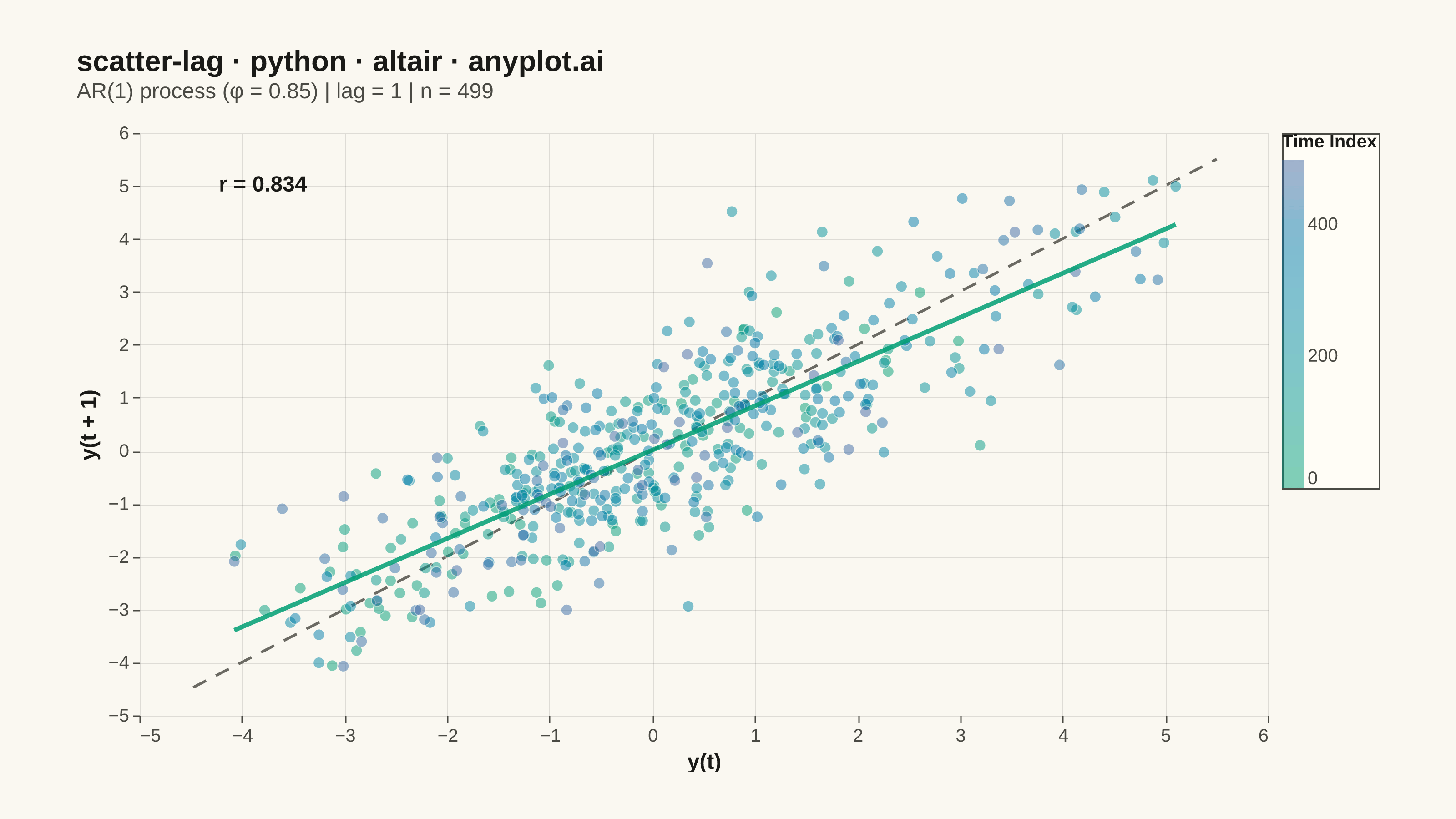
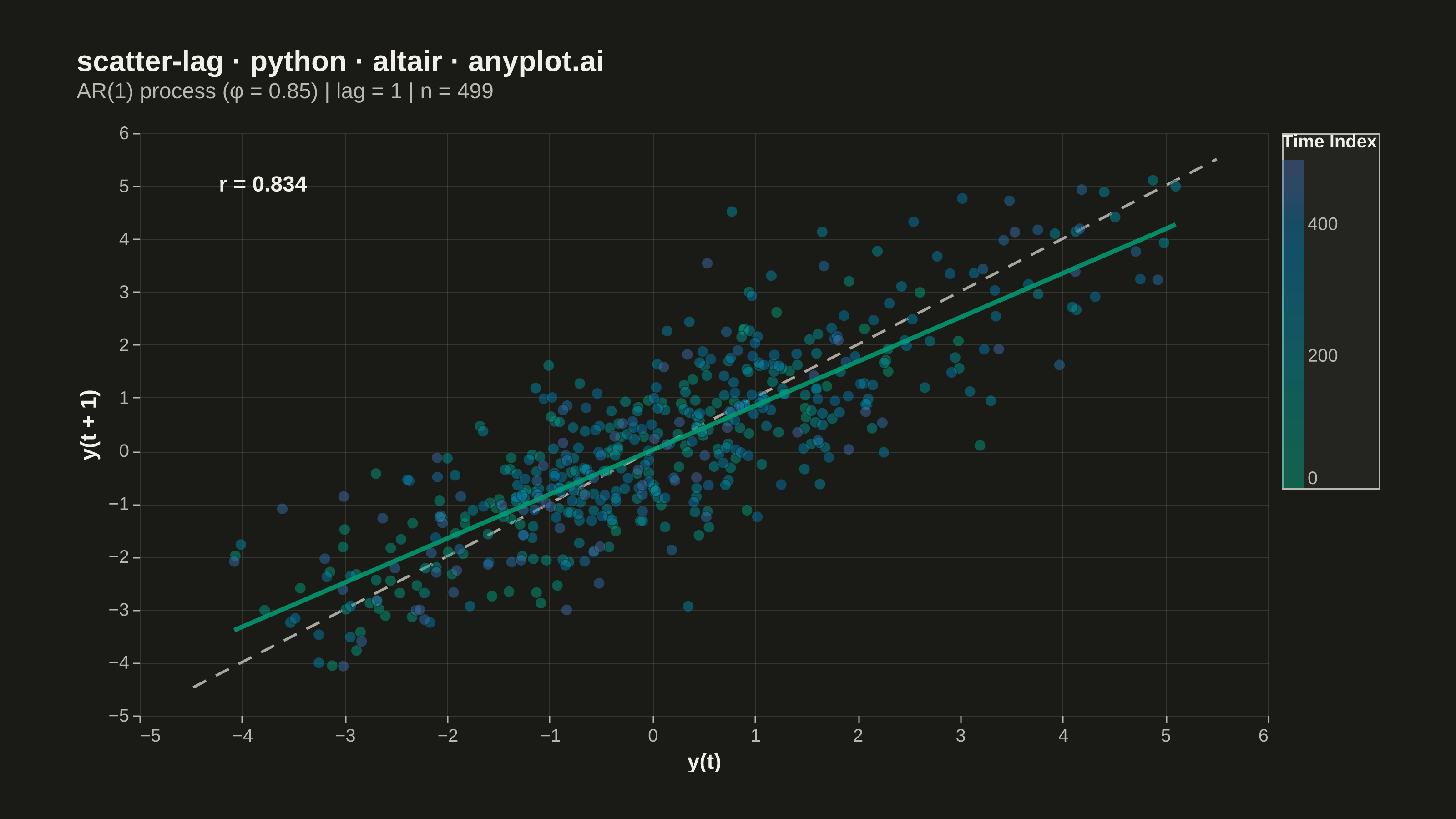
A lag plot is a scatter plot of a time series against a lagged version of itself, plotting y(t) on the x-axis versus y(t+k) on the y-axis for a given lag order k. If the data is purely random, points scatter uniformly with no visible structure; if autocorrelation is present, distinctive patterns emerge — linear clusters for autoregressive processes, elliptical shapes for seasonal data. This provides a quick visual diagnostic for time series dependence, complementing numerical tools like ACF/PACF.
""" anyplot.ai
scatter-lag: Lag Plot for Time Series Autocorrelation Diagnosis
Library: altair 6.2.2 | Python 3.13.14
Quality: 92/100 | Updated: 2026-06-24
"""

import os

import altair as alt
import numpy as np
import pandas as pd
from PIL import Image


# Theme tokens — Imprint palette, theme-adaptive chrome
THEME = os.getenv("ANYPLOT_THEME", "light")
PAGE_BG = "#FAF8F1" if THEME == "light" else "#1A1A17"
ELEVATED_BG = "#FFFDF6" if THEME == "light" else "#242420"
INK = "#1A1A17" if THEME == "light" else "#F0EFE8"
INK_SOFT = "#4A4A44" if THEME == "light" else "#B8B7B0"
INK_MUTED = "#6B6A63" if THEME == "light" else "#A8A79F"
BRAND = "#009E73"  # Imprint palette position 1

# Data — synthetic AR(1) process with strong positive autocorrelation
np.random.seed(42)
n_points = 500
lag = 1
phi = 0.85
noise = np.random.normal(0, 1, n_points)
values = np.zeros(n_points)
values[0] = noise[0]
for i in range(1, n_points):
    values[i] = phi * values[i - 1] + noise[i]

y_t = values[:-lag]
y_t_lag = values[lag:]
r_value = np.corrcoef(y_t, y_t_lag)[0, 1]

df = pd.DataFrame({"y_t": y_t, "y_t_lag": y_t_lag, "time_index": np.arange(n_points - lag)})

# Axis domain with margin
margin = 0.4
axis_min = min(df["y_t"].min(), df["y_t_lag"].min()) - margin
axis_max = max(df["y_t"].max(), df["y_t_lag"].max()) + margin
domain = [axis_min, axis_max]

# Reference line (y = x diagonal — perfect persistence baseline)
ref_df = pd.DataFrame({"x": [axis_min, axis_max], "y": [axis_min, axis_max]})

# Correlation annotation (top-left, away from the dense cluster)
annot_df = pd.DataFrame({"x": [axis_min + 0.25], "y": [axis_max - 0.3], "label": [f"r = {r_value:.3f}"]})

title_str = "scatter-lag · python · altair · anyplot.ai"
subtitle_str = f"AR(1) process (φ = {phi}) | lag = {lag} | n = {n_points - lag}"

# Chart layers
reference_line = (
    alt.Chart(ref_df).mark_line(strokeDash=[8, 6], strokeWidth=1.5, color=INK_MUTED).encode(x="x:Q", y="y:Q")
)

points = (
    alt.Chart(df)
    .mark_point(size=40, filled=True, strokeWidth=0.5, stroke=PAGE_BG, opacity=0.5)
    .encode(
        x=alt.X("y_t:Q", title="y(t)", scale=alt.Scale(domain=domain), axis=alt.Axis(tickCount=8)),
        y=alt.Y("y_t_lag:Q", title="y(t + 1)", scale=alt.Scale(domain=domain), axis=alt.Axis(tickCount=8)),
        # Imprint sequential colormap: brand green → blue (single-polarity continuous)
        color=alt.Color(
            "time_index:Q",
            scale=alt.Scale(range=["#009E73", "#4467A3"]),
            legend=alt.Legend(
                title="Time Index",
                titleFontSize=10,
                labelFontSize=10,
                gradientLength=180,
                gradientThickness=12,
                orient="right",
                offset=8,
            ),
        ),
        tooltip=[
            alt.Tooltip("y_t:Q", title="y(t)", format=".2f"),
            alt.Tooltip("y_t_lag:Q", title="y(t+1)", format=".2f"),
            alt.Tooltip("time_index:Q", title="Time Index"),
        ],
    )
)

# OLS regression line — slope ≈ φ, contrasts with the y=x diagonal to show autocorrelation strength
regression_line = (
    alt.Chart(df)
    .transform_regression("y_t", "y_t_lag", method="linear")
    .mark_line(strokeWidth=2.5, color=BRAND, opacity=0.85)
    .encode(x="y_t:Q", y="y_t_lag:Q")
)

annotation = (
    alt.Chart(annot_df)
    .mark_text(align="left", baseline="top", fontSize=12, fontWeight="bold", color=INK)
    .encode(x="x:Q", y="y:Q", text="label:N")
)

chart = (
    (reference_line + points + regression_line + annotation)
    .properties(
        width=620,
        height=320,
        background=PAGE_BG,
        padding={"left": 0, "right": 0, "top": 0, "bottom": 0},
        title=alt.Title(title_str, fontSize=16, subtitle=subtitle_str, subtitleFontSize=12, subtitleColor=INK_SOFT),
    )
    .configure_view(fill=PAGE_BG, strokeWidth=0, continuousWidth=620, continuousHeight=320)
    .configure_axis(
        labelFontSize=10,
        titleFontSize=12,
        grid=True,
        gridOpacity=0.12,
        gridWidth=0.5,
        gridColor=INK,
        domainWidth=0,
        tickSize=4,
        tickWidth=0.8,
        tickColor=INK_SOFT,
        labelColor=INK_SOFT,
        titleColor=INK,
    )
    .configure_title(anchor="start", offset=12, color=INK)
    .configure_legend(fillColor=ELEVATED_BG, strokeColor=INK_SOFT, labelColor=INK_SOFT, titleColor=INK)
)

# Save PNG + HTML
chart.save(f"plot-{THEME}.png", scale_factor=4.0)
chart.save(f"plot-{THEME}.html")

# Pad PNG to exact 3200×1800 (altair canvas hard contract)
TW, TH = 3200, 1800
_img = Image.open(f"plot-{THEME}.png").convert("RGB")
_w, _h = _img.size
if _w > TW or _h > TH:
    raise SystemExit(
        f"altair vl-convert produced {_w}×{_h}, exceeds target {TW}×{TH}. "
        f"Shrink chart .properties(width=, height=) values and re-render."
    )
if _w < TW or _h < TH:
    _canvas = Image.new("RGB", (TW, TH), PAGE_BG)
    _canvas.paste(_img, ((TW - _w) // 2, (TH - _h) // 2))
    _canvas.save(f"plot-{THEME}.png")
Runnable source as JSON, for any HTTP client: https://api.anyplot.ai/specs/scatter-lag/altair/code. Any spec id and library id listed in llms-full.txt fit the same URL shape; every URL below is complete and callable.
{
  "spec_id": "scatter-lag",
  "language": "python",
  "library": "altair",
  "page": "https://anyplot.ai/scatter-lag/python/altair",
  "hub": "https://anyplot.ai/scatter-lag",
  "code_json": "https://api.anyplot.ai/specs/scatter-lag/altair/code",
  "spec_json": "https://api.anyplot.ai/specs/scatter-lag",
  "render_light_png": "https://storage.googleapis.com/anyplot-images/plots/scatter-lag/python/altair/plot-light.png",
  "render_dark_png": "https://storage.googleapis.com/anyplot-images/plots/scatter-lag/python/altair/plot-dark.png",
  "interactive_light_html": "https://storage.googleapis.com/anyplot-images/plots/scatter-lag/python/altair/plot-light.html",
  "interactive_dark_html": "https://storage.googleapis.com/anyplot-images/plots/scatter-lag/python/altair/plot-dark.html",
  "quality_score": 92.0,
  "license": "MIT",
  "guide": "https://anyplot.ai/llms.txt"
}
Part of Lag Plot for Time Series Autocorrelation Diagnosis on anyplot.ai.