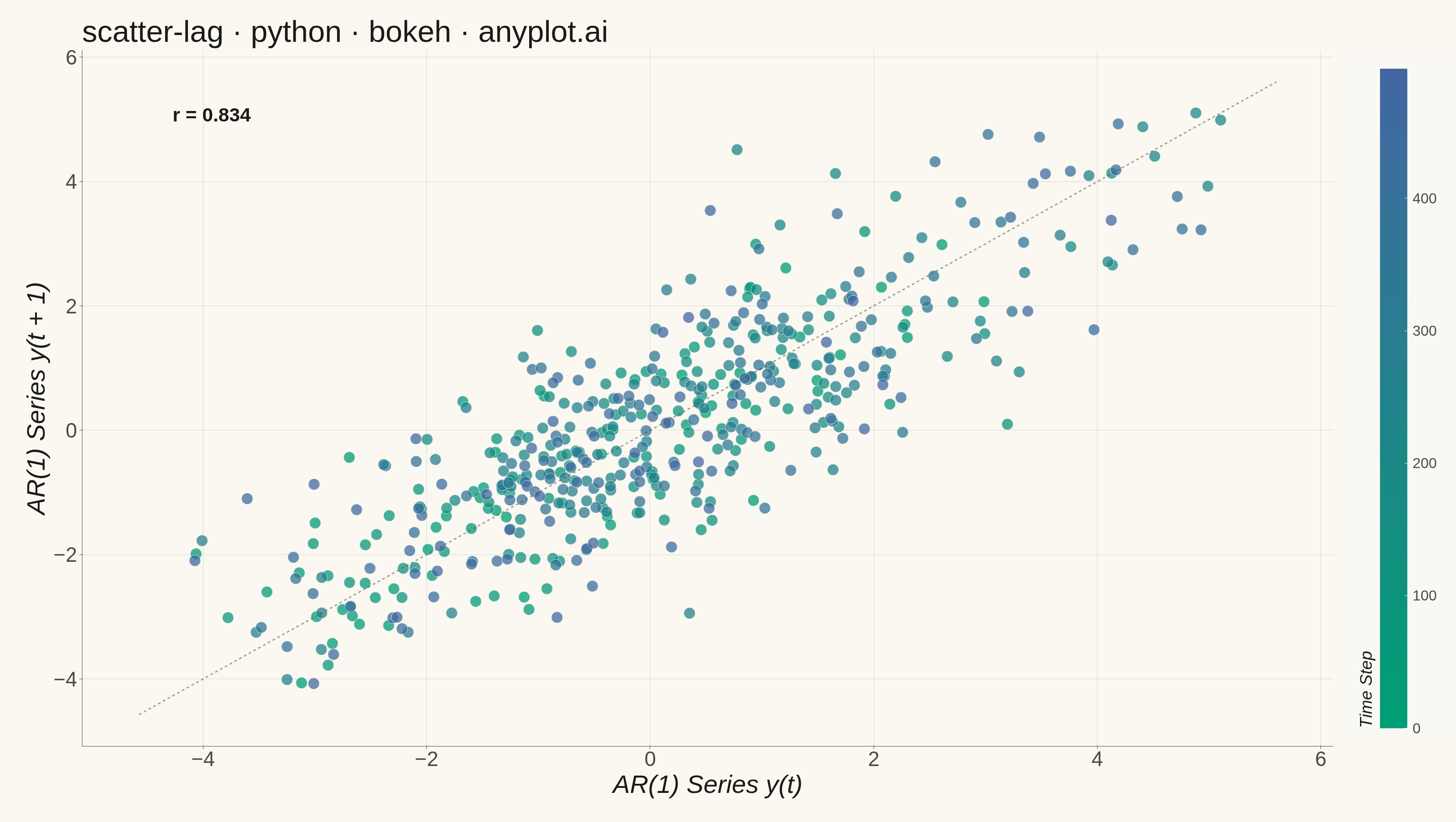
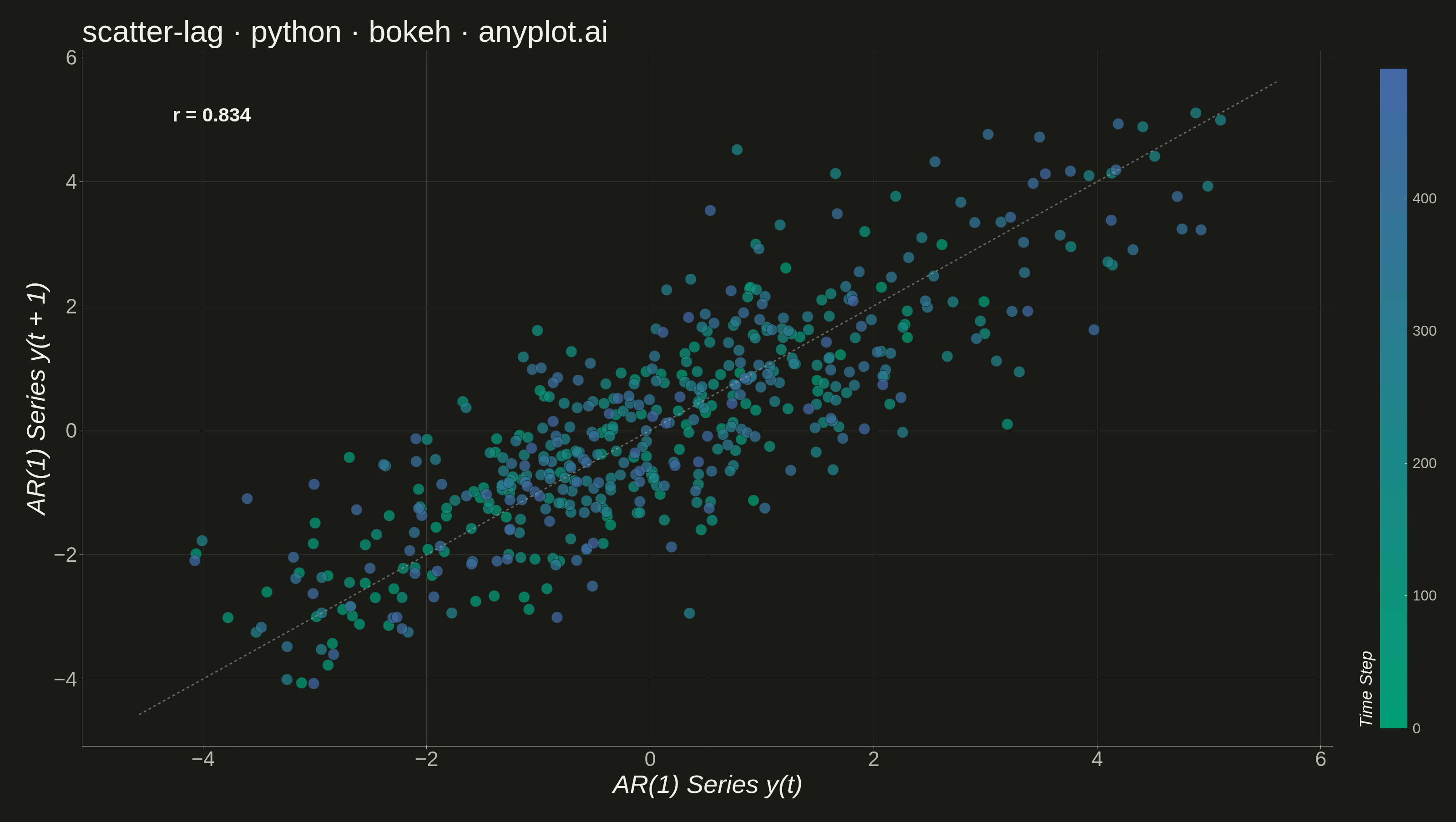
A lag plot is a scatter plot of a time series against a lagged version of itself, plotting y(t) on the x-axis versus y(t+k) on the y-axis for a given lag order k. If the data is purely random, points scatter uniformly with no visible structure; if autocorrelation is present, distinctive patterns emerge — linear clusters for autoregressive processes, elliptical shapes for seasonal data. This provides a quick visual diagnostic for time series dependence, complementing numerical tools like ACF/PACF.
""" anyplot.ai
scatter-lag: Lag Plot for Time Series Autocorrelation Diagnosis
Library: bokeh 3.9.1 | Python 3.13.14
Quality: 90/100 | Updated: 2026-06-24
"""

import os
import sys


# Prevent self-import: this file is named bokeh.py which shadows the installed
# bokeh package when its directory is at the front of sys.path.
_this_dir = os.path.dirname(os.path.abspath(__file__))
sys.path = [p for p in sys.path if os.path.abspath(p or ".") != _this_dir]

import time
from pathlib import Path

import numpy as np
from bokeh.io import output_file, save
from bokeh.models import ColorBar, ColumnDataSource, HoverTool, Label, LinearColorMapper
from bokeh.plotting import figure
from bokeh.transform import linear_cmap
from selenium import webdriver
from selenium.webdriver.chrome.options import Options


# Theme tokens (Imprint palette — see prompts/default-style-guide.md)
THEME = os.getenv("ANYPLOT_THEME", "light")
PAGE_BG = "#FAF8F1" if THEME == "light" else "#1A1A17"
INK = "#1A1A17" if THEME == "light" else "#F0EFE8"
INK_SOFT = "#4A4A44" if THEME == "light" else "#B8B7B0"

# Imprint sequential colormap for time index (single-polarity: green → blue)
_seq = np.round(np.linspace([0x00, 0x9E, 0x73], [0x44, 0x67, 0xA3], 256)).astype(int)
IMPRINT_SEQ256 = ["#{:02X}{:02X}{:02X}".format(*row) for row in _seq]
del _seq

# Data — AR(1) process with strong positive autocorrelation (phi=0.85)
np.random.seed(42)
n_obs = 500
phi = 0.85
noise = np.random.normal(0, 1, n_obs)
series = np.zeros(n_obs)
series[0] = noise[0]
for i in range(1, n_obs):
    series[i] = phi * series[i - 1] + noise[i]

lag = 1
y_t = series[:-lag]
y_t_lag = series[lag:]
time_index = np.arange(len(y_t))
correlation = np.corrcoef(y_t, y_t_lag)[0, 1]

source = ColumnDataSource(data={"y_t": y_t, "y_t_lag": y_t_lag, "time_index": time_index})

# Plot
title = "scatter-lag · python · bokeh · anyplot.ai"

p = figure(
    width=3200,
    height=1800,
    title=title,
    x_axis_label="AR(1) Series y(t)",
    y_axis_label="AR(1) Series y(t + 1)",
    toolbar_location=None,
    min_border_bottom=160,
    min_border_left=180,
    min_border_top=110,
    min_border_right=200,
)

cmap = linear_cmap("time_index", palette=IMPRINT_SEQ256, low=time_index.min(), high=time_index.max())

p.scatter(
    x="y_t", y="y_t_lag", source=source, size=25, fill_color=cmap, line_color=PAGE_BG, line_width=0.8, fill_alpha=0.75
)

# Diagonal reference line (y = x)
axis_min = min(y_t.min(), y_t_lag.min()) - 0.5
axis_max = max(y_t.max(), y_t_lag.max()) + 0.5
p.line(
    [axis_min, axis_max], [axis_min, axis_max], line_color=INK_SOFT, line_dash="dashed", line_width=3, line_alpha=0.5
)

# Color bar for temporal progression
color_mapper = LinearColorMapper(palette=IMPRINT_SEQ256, low=time_index.min(), high=time_index.max())
color_bar = ColorBar(
    color_mapper=color_mapper,
    title="Time Step",
    title_text_font_size="28pt",
    title_text_color=INK,
    title_standoff=20,
    major_label_text_font_size="24pt",
    major_label_text_color=INK_SOFT,
    label_standoff=12,
    width=60,
    padding=40,
    background_fill_color=PAGE_BG,
)
p.add_layout(color_bar, "right")

# Correlation annotation
corr_label = Label(
    x=axis_min + 0.3,
    y=axis_max - 0.7,
    text=f"r = {correlation:.3f}",
    text_font_size="32pt",
    text_color=INK,
    text_font_style="bold",
)
p.add_layout(corr_label)

# HoverTool — distinctive Bokeh interactive feature (active in HTML export)
hover = HoverTool(tooltips=[("y(t)", "@y_t{0.000}"), ("y(t + 1)", "@y_t_lag{0.000}"), ("Time step", "@time_index")])
p.add_tools(hover)

# Style — canonical font sizes for 3200×1800 (see prompts/library/bokeh.md)
p.title.text_font_size = "50pt"
p.title.text_font_style = "normal"
p.title.text_color = INK

p.xaxis.axis_label_text_font_size = "42pt"
p.yaxis.axis_label_text_font_size = "42pt"
p.xaxis.axis_label_text_color = INK
p.yaxis.axis_label_text_color = INK

p.xaxis.major_label_text_font_size = "34pt"
p.yaxis.major_label_text_font_size = "34pt"
p.xaxis.major_label_text_color = INK_SOFT
p.yaxis.major_label_text_color = INK_SOFT

p.xaxis.axis_line_color = INK_SOFT
p.yaxis.axis_line_color = INK_SOFT
p.xaxis.major_tick_line_color = INK_SOFT
p.yaxis.major_tick_line_color = INK_SOFT
p.xaxis.minor_tick_line_color = None
p.yaxis.minor_tick_line_color = None

p.xgrid.grid_line_color = INK
p.ygrid.grid_line_color = INK
p.xgrid.grid_line_alpha = 0.15
p.ygrid.grid_line_alpha = 0.15

p.outline_line_color = None
p.background_fill_color = PAGE_BG
p.border_fill_color = PAGE_BG

# Save HTML (interactive catalog artifact) then PNG via headless Chrome
output_file(f"plot-{THEME}.html")
save(p)

W, H = 3200, 1800
WIN_H = H + 150  # browser viewport offset buffer
opts = Options()
for arg in (
    "--headless=new",
    "--no-sandbox",
    "--disable-dev-shm-usage",
    "--disable-gpu",
    f"--window-size={W},{WIN_H}",
    "--hide-scrollbars",
):
    opts.add_argument(arg)
driver = webdriver.Chrome(options=opts)
driver.set_window_size(W, WIN_H)
driver.get(f"file://{Path(f'plot-{THEME}.html').resolve()}")
time.sleep(3)
driver.execute_script(
    "document.body.style.backgroundColor = arguments[0];document.documentElement.style.backgroundColor = arguments[0];",
    PAGE_BG,
)
time.sleep(1)
driver.save_screenshot(f"plot-{THEME}.png")
driver.quit()
Runnable source as JSON, for any HTTP client: https://api.anyplot.ai/specs/scatter-lag/bokeh/code. Any spec id and library id listed in llms-full.txt fit the same URL shape; every URL below is complete and callable.
{
  "spec_id": "scatter-lag",
  "language": "python",
  "library": "bokeh",
  "page": "https://anyplot.ai/scatter-lag/python/bokeh",
  "hub": "https://anyplot.ai/scatter-lag",
  "code_json": "https://api.anyplot.ai/specs/scatter-lag/bokeh/code",
  "spec_json": "https://api.anyplot.ai/specs/scatter-lag",
  "render_light_png": "https://storage.googleapis.com/anyplot-images/plots/scatter-lag/python/bokeh/plot-light.png",
  "render_dark_png": "https://storage.googleapis.com/anyplot-images/plots/scatter-lag/python/bokeh/plot-dark.png",
  "interactive_light_html": "https://storage.googleapis.com/anyplot-images/plots/scatter-lag/python/bokeh/plot-light.html",
  "interactive_dark_html": "https://storage.googleapis.com/anyplot-images/plots/scatter-lag/python/bokeh/plot-dark.html",
  "quality_score": 90.0,
  "license": "MIT",
  "guide": "https://anyplot.ai/llms.txt"
}
Part of Lag Plot for Time Series Autocorrelation Diagnosis on anyplot.ai.