The same plot in 14 other libraries — Python: Altair, Bokeh, lets-plot, Matplotlib, Plotly, plotnine, Pygal, Seaborn; R: ggplot2; JavaScript: Chart.js, D3.js, Apache ECharts, Highcharts, MUI X Charts. Compare all 15 side by side: Lag Plot for Time Series Autocorrelation Diagnosis in Python, R, Julia and JavaScript.
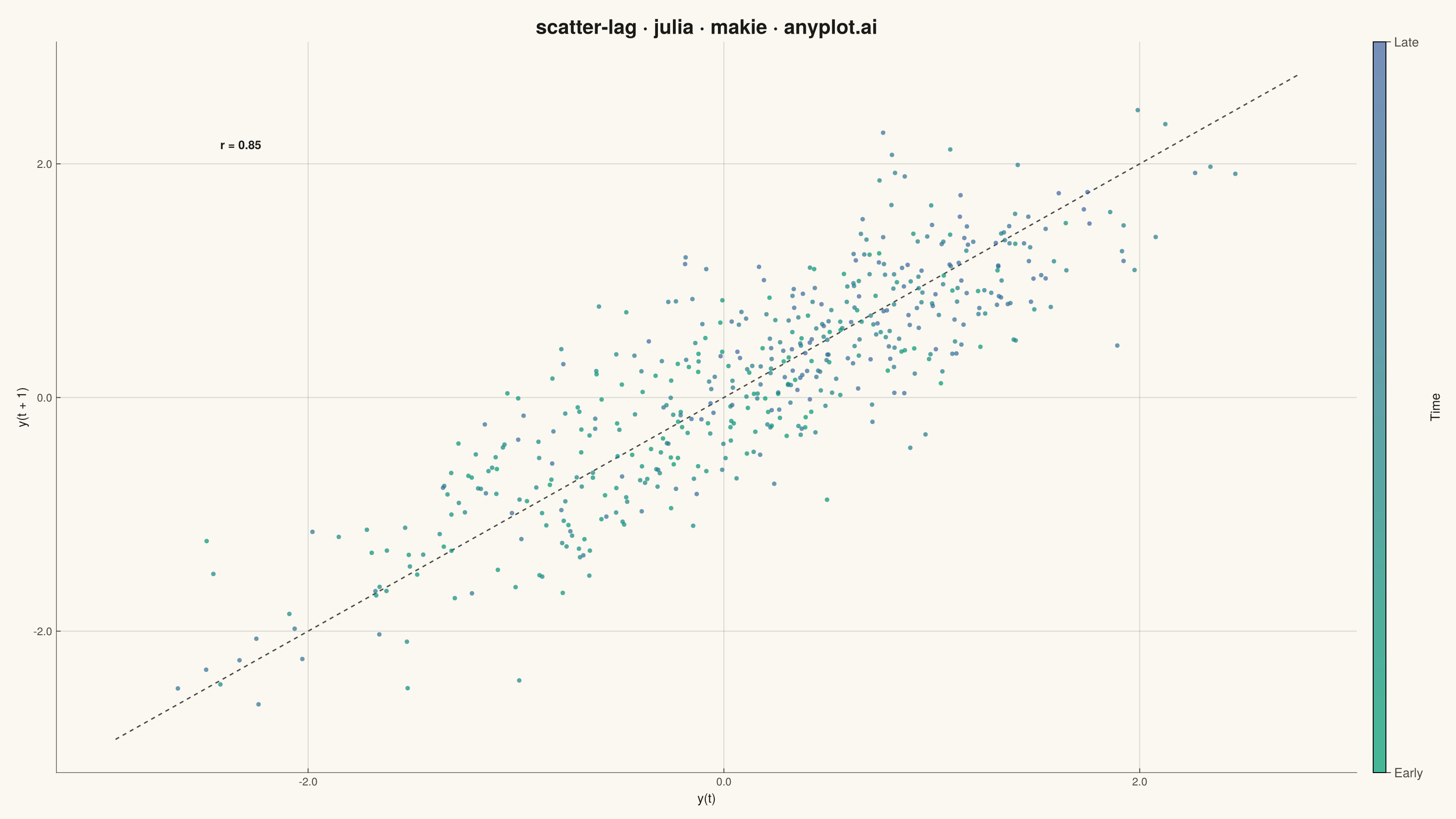
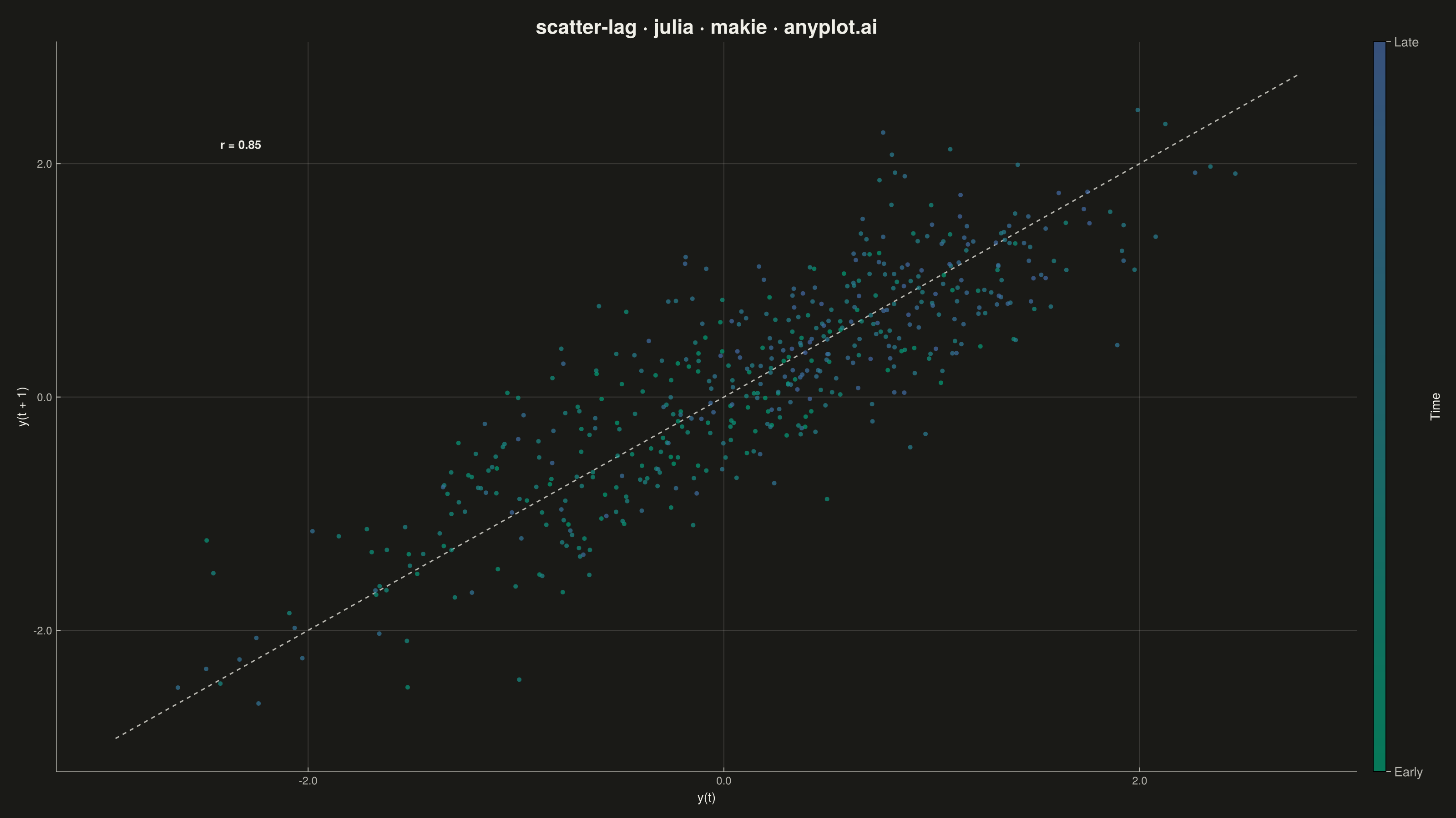
A lag plot is a scatter plot of a time series against a lagged version of itself, plotting y(t) on the x-axis versus y(t+k) on the y-axis for a given lag order k. If the data is purely random, points scatter uniformly with no visible structure; if autocorrelation is present, distinctive patterns emerge — linear clusters for autoregressive processes, elliptical shapes for seasonal data. This provides a quick visual diagnostic for time series dependence, complementing numerical tools like ACF/PACF.
# anyplot.ai
# scatter-lag: Lag Plot for Time Series Autocorrelation Diagnosis
# Library: makie 0.21.9 | Julia 1.11.9
# Quality: 88/100 | Created: 2026-06-24

using CairoMakie
using Colors
using ColorSchemes
using Random
using Statistics

Random.seed!(42)

# Theme tokens (Imprint palette — see prompts/default-style-guide.md)
const THEME    = get(ENV, "ANYPLOT_THEME", "light")
const PAGE_BG  = THEME == "light" ? colorant"#FAF8F1" : colorant"#1A1A17"
const INK      = THEME == "light" ? colorant"#1A1A17" : colorant"#F0EFE8"
const INK_SOFT = THEME == "light" ? colorant"#4A4A44" : colorant"#B8B7B0"

# Sequential Imprint colormap for time-index coloring (green → blue)
const ANYPLOT_SEQ = cgrad([colorant"#009E73", colorant"#4467A3"])

# Makie-distinctive: base theme for tick alignment and spine weight
const ANYPLOT_MAKIE_THEME = Theme(
    Axis = (
        xtickalign = 1,
        ytickalign = 1,
        spinewidth  = 0.7,
    ),
)

# Data: AR(1) process with positive autocorrelation (phi = 0.85)
n = 500
phi = 0.85
ts = zeros(n)
ts[1] = randn()
for i in 2:n
    ts[i] = phi * ts[i-1] + 0.5 * randn()
end

# Lag-1 scatter preparation
lag = 1
y_t  = ts[1:end-lag]
y_t1 = ts[1+lag:end]
n_pts = length(y_t)

# Normalize time index to [0, 1] for sequential color mapping
time_color = collect(1:n_pts) ./ n_pts

# Pearson correlation coefficient at lag 1
r_val = cor(y_t, y_t1)

with_theme(ANYPLOT_MAKIE_THEME) do
    fig = Figure(
        size            = (1600, 900),
        fontsize        = 14,
        backgroundcolor = PAGE_BG,
    )

    ax = Axis(
        fig[1, 1];
        title              = "scatter-lag · julia · makie · anyplot.ai",
        titlesize          = 22,
        titlecolor         = INK,
        xlabel             = "y(t)",
        ylabel             = "y(t + 1)",
        xlabelsize         = 14,
        ylabelsize         = 14,
        xlabelcolor        = INK,
        ylabelcolor        = INK,
        xticklabelsize     = 12,
        yticklabelsize     = 12,
        xticklabelcolor    = INK_SOFT,
        yticklabelcolor    = INK_SOFT,
        xtickcolor         = INK_SOFT,
        ytickcolor         = INK_SOFT,
        backgroundcolor    = PAGE_BG,
        topspinevisible    = false,
        rightspinevisible  = false,
        leftspinecolor     = INK_SOFT,
        bottomspinecolor   = INK_SOFT,
        xgridcolor         = RGBAf(INK.r, INK.g, INK.b, 0.15),
        ygridcolor         = RGBAf(INK.r, INK.g, INK.b, 0.15),
        xminorgridvisible  = false,
        yminorgridvisible  = false,
        xtickformat        = values -> ["$(round(v; digits=1))" for v in values],
        ytickformat        = values -> ["$(round(v; digits=1))" for v in values],
    )

    # Diagonal reference line y = x
    all_vals = vcat(y_t, y_t1)
    lo = minimum(all_vals) - 0.3
    hi = maximum(all_vals) + 0.3
    ref_line = range(lo, hi; length = 100)
    lines!(ax, collect(ref_line), collect(ref_line);
        color     = INK_SOFT,
        linewidth = 1.5,
        linestyle = :dash,
    )

    # Scatter colored by time index using the Imprint sequential colormap
    sc = scatter!(ax, y_t, y_t1;
        color       = time_color,
        colormap    = ANYPLOT_SEQ,
        colorrange  = (0.0, 1.0),
        markersize  = 7,
        alpha       = 0.72,
        strokewidth = 0,
    )

    # Colorbar labeling the temporal axis
    Colorbar(fig[1, 2], sc;
        label          = "Time",
        labelcolor     = INK,
        tickcolor      = INK_SOFT,
        ticklabelcolor = INK_SOFT,
        width          = 14,
        tellheight     = false,
        ticks          = ([0.0, 1.0], ["Early", "Late"]),
    )

    # Correlation coefficient annotation in data coordinates
    ann_x = minimum(y_t)  + 0.04 * (maximum(y_t)  - minimum(y_t))
    ann_y = minimum(y_t1) + 0.93 * (maximum(y_t1) - minimum(y_t1))
    text!(ax, "r = $(round(r_val; digits = 2))";
        position = (ann_x, ann_y),
        fontsize = 13,
        color    = INK,
        font     = :bold,
    )

    # Save
    save("plot-$(THEME).png", fig; px_per_unit = 2)
end
Runnable source as JSON, for any HTTP client: https://api.anyplot.ai/specs/scatter-lag/makie/code. Any spec id and library id listed in llms-full.txt fit the same URL shape; every URL below is complete and callable.
{
  "spec_id": "scatter-lag",
  "language": "julia",
  "library": "makie",
  "page": "https://anyplot.ai/scatter-lag/julia/makie",
  "hub": "https://anyplot.ai/scatter-lag",
  "code_json": "https://api.anyplot.ai/specs/scatter-lag/makie/code",
  "spec_json": "https://api.anyplot.ai/specs/scatter-lag",
  "render_light_png": "https://storage.googleapis.com/anyplot-images/plots/scatter-lag/julia/makie/plot-light.png",
  "render_dark_png": "https://storage.googleapis.com/anyplot-images/plots/scatter-lag/julia/makie/plot-dark.png",
  "quality_score": 88.0,
  "license": "MIT",
  "guide": "https://anyplot.ai/llms.txt"
}
Part of Lag Plot for Time Series Autocorrelation Diagnosis on anyplot.ai.