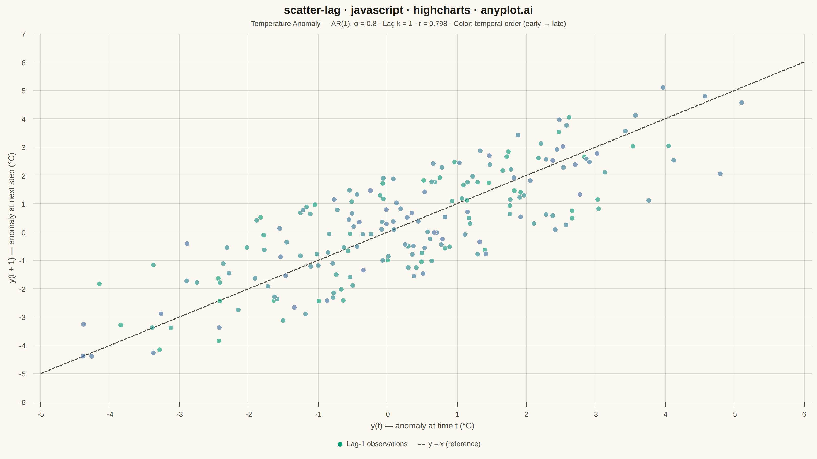
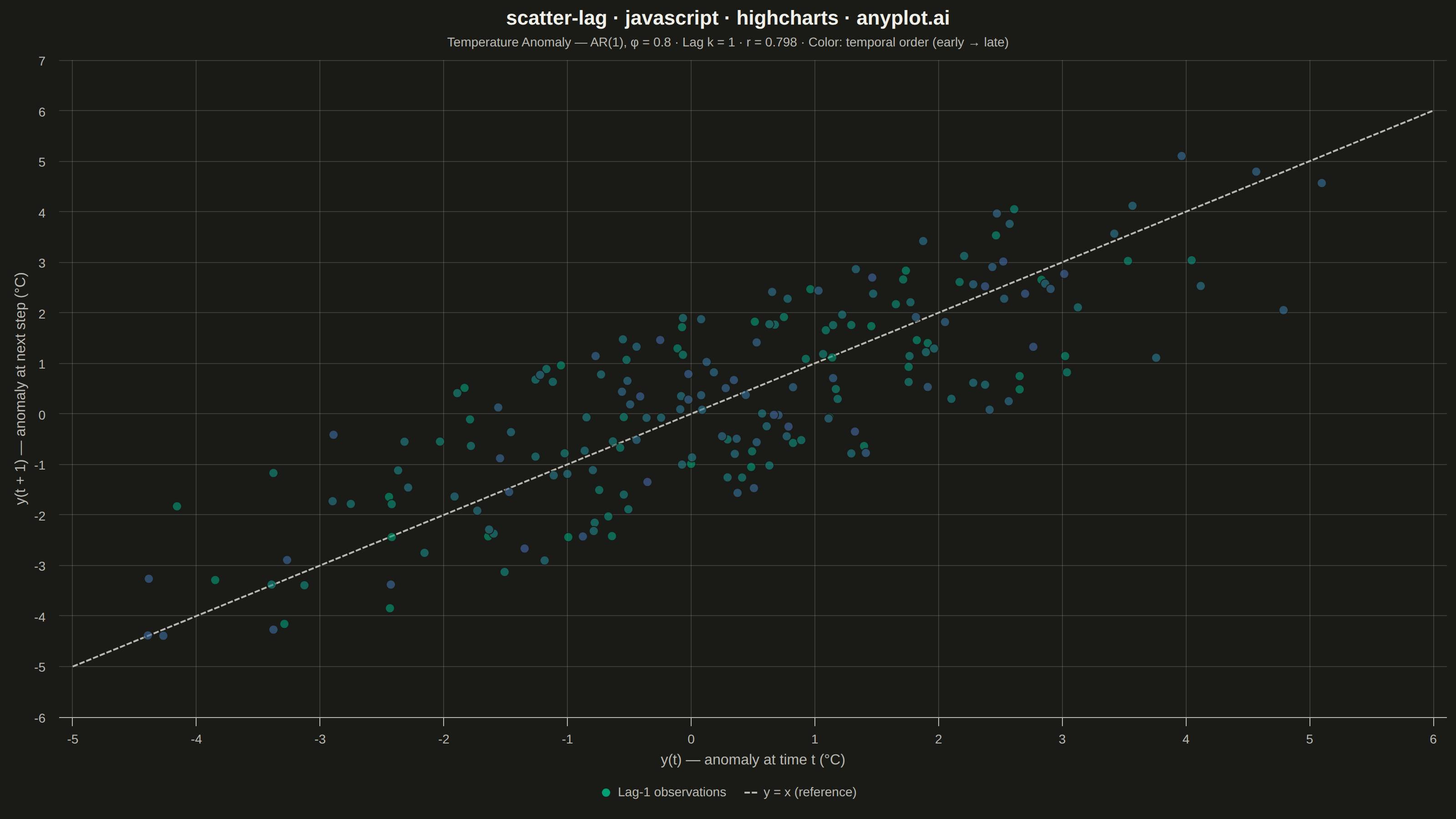
The same plot in 14 other libraries — JavaScript: Chart.js, D3.js, Apache ECharts, MUI X Charts; Python: Altair, Bokeh, lets-plot, Matplotlib, Plotly, plotnine, Pygal, Seaborn; R: ggplot2; Julia: Makie.jl. Compare all 15 side by side: Lag Plot for Time Series Autocorrelation Diagnosis in Python, R, Julia and JavaScript.
A lag plot is a scatter plot of a time series against a lagged version of itself, plotting y(t) on the x-axis versus y(t+k) on the y-axis for a given lag order k. If the data is purely random, points scatter uniformly with no visible structure; if autocorrelation is present, distinctive patterns emerge — linear clusters for autoregressive processes, elliptical shapes for seasonal data. This provides a quick visual diagnostic for time series dependence, complementing numerical tools like ACF/PACF.
// anyplot.ai
// scatter-lag: Lag Plot for Time Series Autocorrelation Diagnosis
// Library: highcharts 12.6.0 | JavaScript 22.22.3
// Quality: 91/100 | Created: 2026-06-24

//# anyplot-orientation: landscape

const t = window.ANYPLOT_TOKENS;

// Deterministic LCG for reproducible synthetic data (seed = 42)
let _s = 42;
function rng() {
  _s = (_s * 1664525 + 1013904223) >>> 0;
  return _s / 4294967295;
}

// AR(1) time series: y(t) = phi * y(t-1) + epsilon
const nObs = 200;
const phi = 0.8;
const ts = [0.0];
for (let i = 1; i < nObs; i++) {
  ts.push(phi * ts[i - 1] + (rng() - 0.5) * 4);
}

// Lag-1 scatter: x = y(t), y = y(t + 1)
const lag = 1;
const xVals = ts.slice(0, nObs - lag);
const yVals = ts.slice(lag);
const nPairs = xVals.length;

// Pearson lag-1 autocorrelation coefficient r
const mx  = xVals.reduce((a, b) => a + b, 0) / nPairs;
const my  = yVals.reduce((a, b) => a + b, 0) / nPairs;
const num = xVals.reduce((s, x, i) => s + (x - mx) * (yVals[i] - my), 0);
const dx  = Math.sqrt(xVals.reduce((s, x) => s + (x - mx) ** 2, 0));
const dy  = Math.sqrt(yVals.reduce((s, y) => s + (y - my) ** 2, 0));
const r   = (num / (dx * dy)).toFixed(3);

// Diagonal reference line extent
const vMin = Math.floor(Math.min(...xVals, ...yVals));
const vMax = Math.ceil(Math.max(...xVals, ...yVals));

// Interpolate between two #RRGGBB hex colors by fraction 0..1
function hexToRgb(hex) {
  return [parseInt(hex.slice(1, 3), 16), parseInt(hex.slice(3, 5), 16), parseInt(hex.slice(5, 7), 16)];
}
function lerpColor(c1, c2, frac) {
  const [r1, g1, b1] = hexToRgb(c1);
  const [r2, g2, b2] = hexToRgb(c2);
  return `rgb(${Math.round(r1 + (r2 - r1) * frac)},${Math.round(g1 + (g2 - g1) * frac)},${Math.round(b1 + (b2 - b1) * frac)})`;
}

// Color each lag pair by temporal position using imprint_seq: early (seq[0]) → late (seq[1])
const scatterPts = xVals.map((x, i) => ({
  x: +x.toFixed(3),
  y: +yVals[i].toFixed(3),
  color: lerpColor(t.seq[0], t.seq[1], i / (nPairs - 1))
}));

Highcharts.chart("container", {
  chart: {
    backgroundColor: "transparent",
    animation: false,
    style: { fontFamily: "inherit" },
    plotBorderWidth: 0
  },
  credits: { enabled: false },
  colors: t.palette,

  title: {
    text: "scatter-lag · javascript · highcharts · anyplot.ai",
    style: { color: t.ink, fontSize: "22px", fontWeight: "600" }
  },
  subtitle: {
    text: "Temperature Anomaly — AR(1), φ = " + phi + " · Lag k = " + lag + " · r = " + r + " · Color: temporal order (early → late)",
    style: { color: t.inkSoft, fontSize: "14px" }
  },

  xAxis: {
    title: {
      text: "y(t) — anomaly at time t (°C)",
      style: { color: t.inkSoft, fontSize: "16px" }
    },
    lineColor: t.inkSoft,
    tickColor: t.inkSoft,
    gridLineColor: t.grid,
    gridLineWidth: 1,
    labels: { style: { color: t.inkSoft, fontSize: "14px" } }
  },
  yAxis: {
    title: {
      text: "y(t + 1) — anomaly at next step (°C)",
      style: { color: t.inkSoft, fontSize: "16px" }
    },
    lineColor: t.inkSoft,
    tickColor: t.inkSoft,
    gridLineColor: t.grid,
    gridLineWidth: 1,
    labels: { style: { color: t.inkSoft, fontSize: "14px" } }
  },

  legend: {
    enabled: true,
    itemStyle: { color: t.inkSoft, fontSize: "14px" },
    itemHoverStyle: { color: t.ink }
  },

  plotOptions: {
    series: { animation: false },
    scatter: {
      marker: {
        radius: 5,
        symbol: "circle",
        lineWidth: 1,
        lineColor: t.pageBg
      },
      opacity: 0.62
    },
    line: {
      marker: { enabled: false },
      enableMouseTracking: false
    }
  },

  series: [
    {
      name: "Lag-1 observations",
      type: "scatter",
      data: scatterPts,
      color: t.palette[0],  // legend marker; individual points use imprint_seq gradient
      zIndex: 2
    },
    {
      name: "y = x (reference)",
      type: "line",
      data: [[vMin, vMin], [vMax, vMax]],
      color: t.inkSoft,
      dashStyle: "ShortDash",
      lineWidth: 2,
      zIndex: 1
    }
  ]
});
Runnable source as JSON, for any HTTP client: https://api.anyplot.ai/specs/scatter-lag/highcharts/code. Any spec id and library id listed in llms-full.txt fit the same URL shape; every URL below is complete and callable.
{
  "spec_id": "scatter-lag",
  "language": "javascript",
  "library": "highcharts",
  "page": "https://anyplot.ai/scatter-lag/javascript/highcharts",
  "hub": "https://anyplot.ai/scatter-lag",
  "code_json": "https://api.anyplot.ai/specs/scatter-lag/highcharts/code",
  "spec_json": "https://api.anyplot.ai/specs/scatter-lag",
  "render_light_png": "https://storage.googleapis.com/anyplot-images/plots/scatter-lag/javascript/highcharts/plot-light.png",
  "render_dark_png": "https://storage.googleapis.com/anyplot-images/plots/scatter-lag/javascript/highcharts/plot-dark.png",
  "interactive_light_html": "https://storage.googleapis.com/anyplot-images/plots/scatter-lag/javascript/highcharts/plot-light.html",
  "interactive_dark_html": "https://storage.googleapis.com/anyplot-images/plots/scatter-lag/javascript/highcharts/plot-dark.html",
  "quality_score": 91.0,
  "license": "MIT",
  "guide": "https://anyplot.ai/llms.txt"
}
Part of Lag Plot for Time Series Autocorrelation Diagnosis on anyplot.ai.