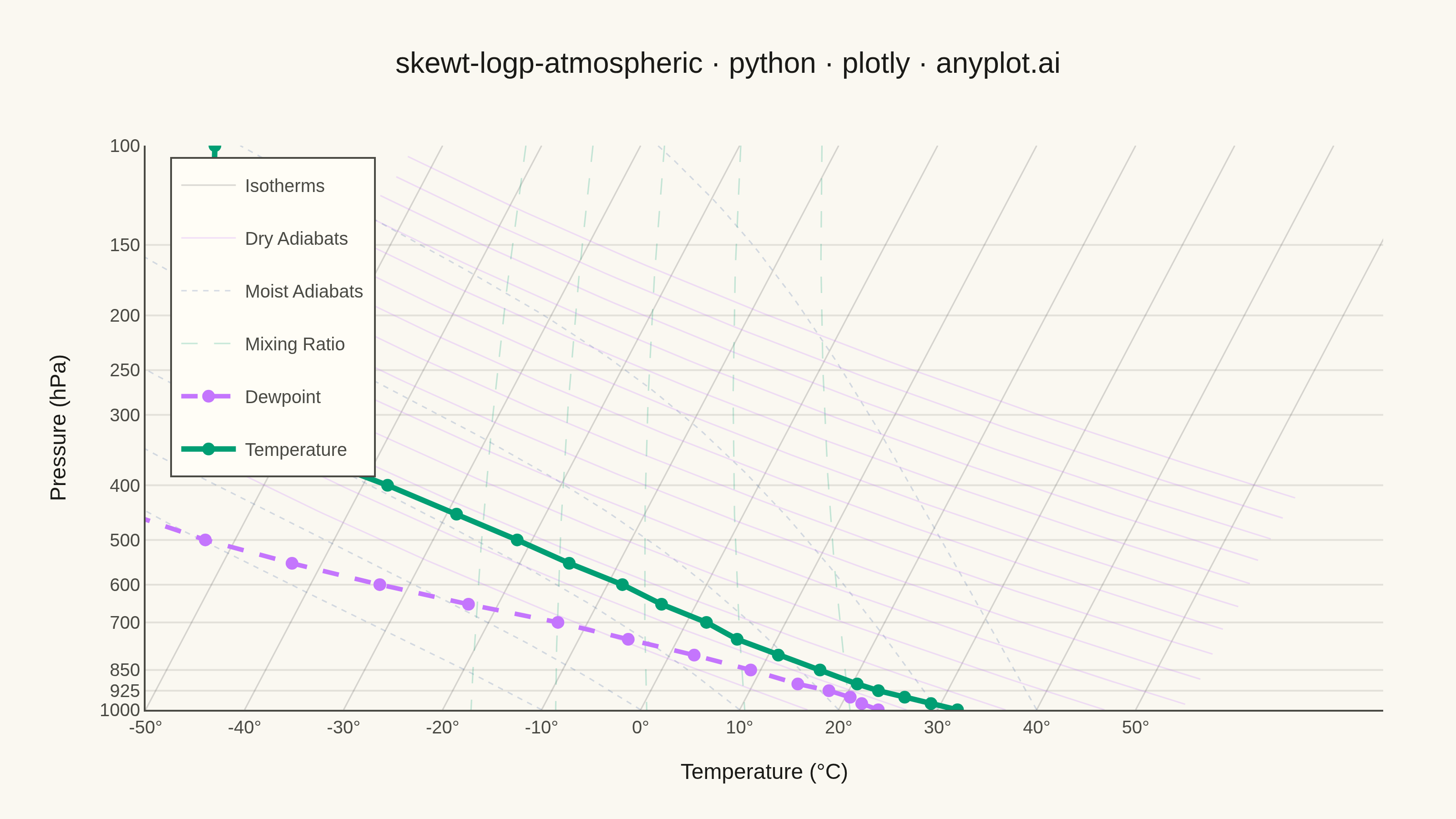
The same plot in 14 other libraries — Python: Altair, Bokeh, lets-plot, Matplotlib, plotnine, Pygal, Seaborn; R: ggplot2; Julia: Makie.jl; JavaScript: Chart.js, D3.js, Apache ECharts, Highcharts, MUI X Charts. Compare all 15 side by side: Skew-T Log-P Atmospheric Diagram in Python, R, Julia and JavaScript.
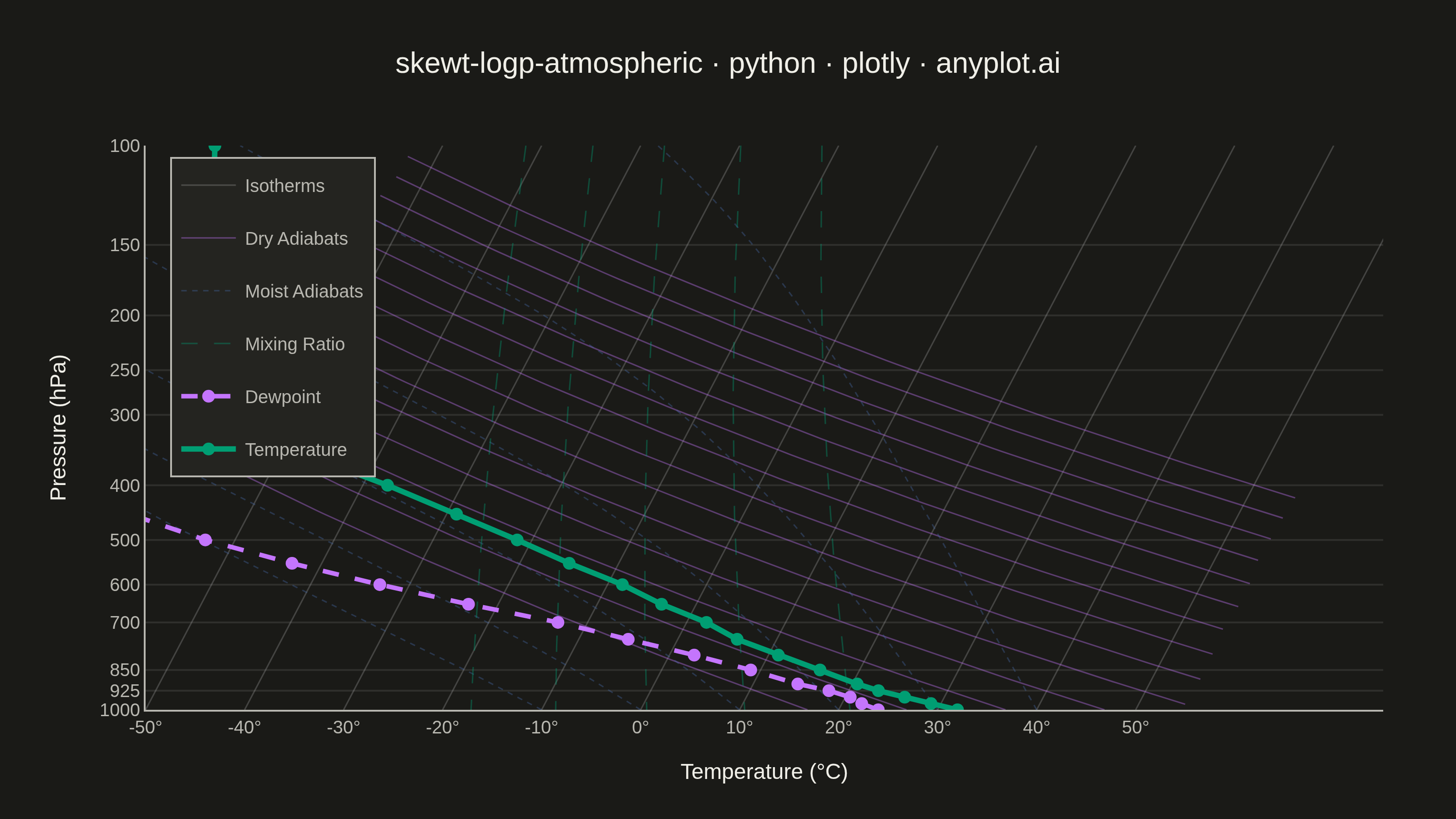
A Skew-T Log-P diagram is a specialized thermodynamic chart used in meteorology to display vertical atmospheric profiles. It features a logarithmic pressure axis (inverted, with surface at bottom) and temperature isotherms skewed 45 degrees to the right, allowing simultaneous visualization of temperature, dewpoint, and derived stability parameters. This diagram is essential for analyzing atmospheric soundings and assessing weather conditions.
""" anyplot.ai
skewt-logp-atmospheric: Skew-T Log-P Atmospheric Diagram
Library: plotly 6.7.0 | Python 3.13.13
Quality: 87/100 | Updated: 2026-05-21
"""

import os

import numpy as np
import plotly.graph_objects as go


# Theme tokens
THEME = os.getenv("ANYPLOT_THEME", "light")
PAGE_BG = "#FAF8F1" if THEME == "light" else "#1A1A17"
ELEVATED_BG = "#FFFDF6" if THEME == "light" else "#242420"
INK = "#1A1A17" if THEME == "light" else "#F0EFE8"
INK_SOFT = "#4A4A44" if THEME == "light" else "#B8B7B0"
GRID = "rgba(26, 26, 23, 0.10)" if THEME == "light" else "rgba(240, 239, 232, 0.10)"

BRAND = "#009E73"  # Okabe-Ito pos 1 — temperature profile
C_DEWPT = "#C475FD"  # Okabe-Ito pos 2 — dewpoint profile

# Reference line colors: subtle, theme-adaptive
C_ISO = "rgba(80, 80, 80, 0.22)" if THEME == "light" else "rgba(180, 180, 180, 0.28)"
C_DRY = "rgba(196, 117, 253, 0.22)" if THEME == "light" else "rgba(196, 117, 253, 0.38)"
C_MOIST = "rgba(68, 103, 163, 0.22)" if THEME == "light" else "rgba(68, 103, 163, 0.38)"
C_MIX = "rgba(0, 158, 115, 0.22)" if THEME == "light" else "rgba(0, 158, 115, 0.38)"

# Skew-T transform: °C shift per log10 decade of pressure from 1000 hPa
SKEW = 30.0


def skew_x(T, P):
    return T + SKEW * np.log10(1000.0 / P)


# Atmospheric constants
Rd = 287.05  # J/(kg·K)
Cp = 1004.0  # J/(kg·K)
Lv = 2.5e6  # J/kg
Rv = 461.5  # J/(kg·K)
Rd_Cp = Rd / Cp  # ≈ 0.2854


def moist_adiabat(T0_C, P_start=1000.0, P_end=100.0, n=150):
    """Integrate moist adiabat from P_start to P_end starting at T0_C."""
    P = np.linspace(P_start, P_end, n)
    T = np.zeros(n)
    T[0] = T0_C
    for i in range(1, n):
        T_K = T[i - 1] + 273.15
        es = 6.112 * np.exp(17.67 * T[i - 1] / (T[i - 1] + 243.5))
        rs = 0.622 * es / max(P[i - 1] - es, 0.001)
        num = Rd * T_K + Lv * rs
        den = P[i - 1] * (Cp + Lv**2 * rs / (Rv * T_K**2))
        T[i] = T[i - 1] + (num / den) * (P[i] - P[i - 1])
    return P, T


# Data: synthetic warm-moist sounding, US Great Plains summer
pressure = np.array(
    [1000, 975, 950, 925, 900, 850, 800, 750, 700, 650, 600, 550, 500, 450, 400, 350, 300, 250, 200, 150, 100]
)
temperature = np.array(
    [
        32.0,
        29.0,
        26.0,
        23.0,
        20.5,
        16.0,
        11.0,
        6.0,
        2.0,
        -3.5,
        -8.5,
        -15.0,
        -21.5,
        -29.0,
        -37.5,
        -48.0,
        -56.0,
        -62.0,
        -64.5,
        -68.0,
        -73.0,
    ]
)
dewpoint = np.array(
    [
        24.0,
        22.0,
        20.5,
        18.0,
        14.5,
        9.0,
        2.5,
        -5.0,
        -13.0,
        -23.0,
        -33.0,
        -43.0,
        -53.0,
        -62.0,
        -70.0,
        -76.0,
        -81.0,
        -84.0,
        -86.0,
        -88.0,
        -90.0,
    ]
)

# Lifting Condensation Level (LCL) — surface parcel T=32°C, Td=24°C
# At DALR=9.8°C/km and dewpoint cooling ~1.8°C/km, they meet at z≈1 km ≈ 900 hPa
LCL_P = 900.0
LCL_T = 22.0

# Pressure array for reference lines
P_ref = np.linspace(100.0, 1000.0, 200)

fig = go.Figure()

# --- Reference lines (background layer) ---

# Isotherms (constant temperature, appear as diagonal lines when skewed)
for idx, T_iso in enumerate(range(-50, 55, 10)):
    fig.add_trace(
        go.Scatter(
            x=skew_x(T_iso * np.ones_like(P_ref), P_ref),
            y=P_ref,
            mode="lines",
            line=dict(color=C_ISO, width=0.8),
            legendgroup="iso",
            showlegend=(idx == 0),
            name="Isotherms",
            hoverinfo="skip",
        )
    )

# Dry adiabats (constant potential temperature θ)
for idx, theta in enumerate(range(290, 430, 10)):
    T_dry = theta * (P_ref / 1000.0) ** Rd_Cp - 273.15
    mask = (T_dry > -55) & (T_dry < 55)
    x_d = np.where(mask, skew_x(T_dry, P_ref), np.nan)
    if not np.all(np.isnan(x_d)):
        fig.add_trace(
            go.Scatter(
                x=x_d,
                y=P_ref,
                mode="lines",
                line=dict(color=C_DRY, width=0.8),
                legendgroup="dry",
                showlegend=(idx == 0),
                name="Dry Adiabats",
                hoverinfo="skip",
            )
        )

# Moist adiabats (saturated adiabatic lapse rate, numerically integrated)
for idx, T0 in enumerate(range(-10, 45, 10)):
    P_m, T_m = moist_adiabat(T0)
    fig.add_trace(
        go.Scatter(
            x=skew_x(T_m, P_m),
            y=P_m,
            mode="lines",
            line=dict(color=C_MOIST, width=0.8, dash="dot"),
            legendgroup="moist",
            showlegend=(idx == 0),
            name="Moist Adiabats",
            hoverinfo="skip",
        )
    )

# Mixing ratio lines (constant water vapor mixing ratio)
for idx, r_gkg in enumerate([1, 2, 4, 8, 16]):
    r = r_gkg / 1000.0
    es = r * P_ref / (r + 0.622)
    with np.errstate(divide="ignore", invalid="ignore"):
        log_r = np.log(es / 6.112)
        T_mix = 243.5 * log_r / (17.67 - log_r)
    mask = np.isfinite(T_mix) & (T_mix > -50) & (T_mix < 35)
    x_mix = np.where(mask, skew_x(T_mix, P_ref), np.nan)
    fig.add_trace(
        go.Scatter(
            x=x_mix,
            y=P_ref,
            mode="lines",
            line=dict(color=C_MIX, width=0.8, dash="dash"),
            legendgroup="mix",
            showlegend=(idx == 0),
            name="Mixing Ratio",
            hoverinfo="skip",
        )
    )

# --- Atmospheric sounding profiles ---

# Dewpoint (dashed blue)
fig.add_trace(
    go.Scatter(
        x=skew_x(dewpoint, pressure),
        y=pressure,
        mode="lines+markers",
        name="Dewpoint",
        line=dict(color=C_DEWPT, width=2.5, dash="dash"),
        marker=dict(color=C_DEWPT, size=7),
        customdata=np.column_stack([dewpoint, pressure]),
        hovertemplate="%{customdata[1]:.0f} hPa | Td: %{customdata[0]:.1f}°C<extra></extra>",
    )
)

# Temperature (solid green, Okabe-Ito pos 1)
fig.add_trace(
    go.Scatter(
        x=skew_x(temperature, pressure),
        y=pressure,
        mode="lines+markers",
        name="Temperature",
        line=dict(color=BRAND, width=3.0),
        marker=dict(color=BRAND, size=7),
        customdata=np.column_stack([temperature, pressure]),
        hovertemplate="%{customdata[1]:.0f} hPa | T: %{customdata[0]:.1f}°C<extra></extra>",
    )
)

# --- Layout ---

# x-axis ticks: at P=1000 hPa, skew=0 so tick position = actual temperature
tick_T = list(range(-50, 55, 10))

fig.update_layout(
    autosize=False,
    paper_bgcolor=PAGE_BG,
    plot_bgcolor=PAGE_BG,
    title=dict(
        text="skewt-logp-atmospheric · python · plotly · anyplot.ai",
        font=dict(size=16, color=INK),
        x=0.5,
        xanchor="center",
    ),
    xaxis=dict(
        title=dict(text="Temperature (°C)", font=dict(size=12, color=INK)),
        tickfont=dict(size=10, color=INK_SOFT),
        linecolor=INK_SOFT,
        zeroline=False,
        showgrid=False,
        tickmode="array",
        tickvals=[float(t) for t in tick_T],
        ticktext=[f"{t}°" for t in tick_T],
        range=[-50.0, 75.0],
    ),
    yaxis=dict(
        title=dict(text="Pressure (hPa)", font=dict(size=12, color=INK)),
        tickfont=dict(size=10, color=INK_SOFT),
        gridcolor=GRID,
        linecolor=INK_SOFT,
        zeroline=False,
        type="log",
        range=[3.0, 2.0],  # log10(1000)=3 at bottom → 1000 hPa, log10(100)=2 at top
        tickmode="array",
        tickvals=[100, 150, 200, 250, 300, 400, 500, 600, 700, 850, 925, 1000],
        ticktext=["100", "150", "200", "250", "300", "400", "500", "600", "700", "850", "925", "1000"],
        showgrid=True,
    ),
    legend=dict(
        bgcolor=ELEVATED_BG,
        bordercolor=INK_SOFT,
        borderwidth=1,
        font=dict(size=10, color=INK_SOFT),
        x=0.02,
        y=0.98,
        xanchor="left",
        yanchor="top",
    ),
    margin=dict(l=80, r=40, t=80, b=60),
    annotations=[
        dict(
            x=skew_x(LCL_T, LCL_P),
            y=LCL_P,
            xref="x",
            yref="y",
            text="LCL ≈ 900 hPa",
            showarrow=True,
            arrowhead=2,
            arrowcolor=INK_SOFT,
            arrowwidth=1.5,
            ax=55,
            ay=-30,
            font=dict(size=10, color=INK),
            bgcolor=ELEVATED_BG,
            bordercolor=INK_SOFT,
            borderwidth=1,
            borderpad=4,
            opacity=0.9,
        )
    ],
)

# Save
fig.write_image(f"plot-{THEME}.png", width=800, height=450, scale=4)
fig.write_html(f"plot-{THEME}.html", include_plotlyjs="cdn")
Runnable source as JSON, for any HTTP client: https://api.anyplot.ai/specs/skewt-logp-atmospheric/plotly/code. Any spec id and library id listed in llms-full.txt fit the same URL shape; every URL below is complete and callable.
{
  "spec_id": "skewt-logp-atmospheric",
  "language": "python",
  "library": "plotly",
  "page": "https://anyplot.ai/skewt-logp-atmospheric/python/plotly",
  "hub": "https://anyplot.ai/skewt-logp-atmospheric",
  "code_json": "https://api.anyplot.ai/specs/skewt-logp-atmospheric/plotly/code",
  "spec_json": "https://api.anyplot.ai/specs/skewt-logp-atmospheric",
  "render_light_png": "https://storage.googleapis.com/anyplot-images/plots/skewt-logp-atmospheric/python/plotly/plot-light.png",
  "render_dark_png": "https://storage.googleapis.com/anyplot-images/plots/skewt-logp-atmospheric/python/plotly/plot-dark.png",
  "interactive_light_html": "https://storage.googleapis.com/anyplot-images/plots/skewt-logp-atmospheric/python/plotly/plot-light.html",
  "interactive_dark_html": "https://storage.googleapis.com/anyplot-images/plots/skewt-logp-atmospheric/python/plotly/plot-dark.html",
  "quality_score": 87.0,
  "license": "MIT",
  "guide": "https://anyplot.ai/llms.txt"
}
Part of Skew-T Log-P Atmospheric Diagram on anyplot.ai.