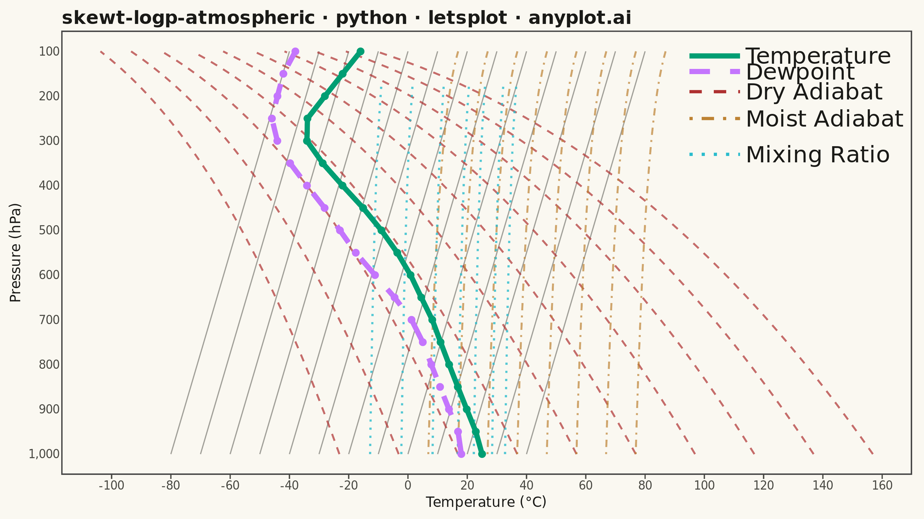
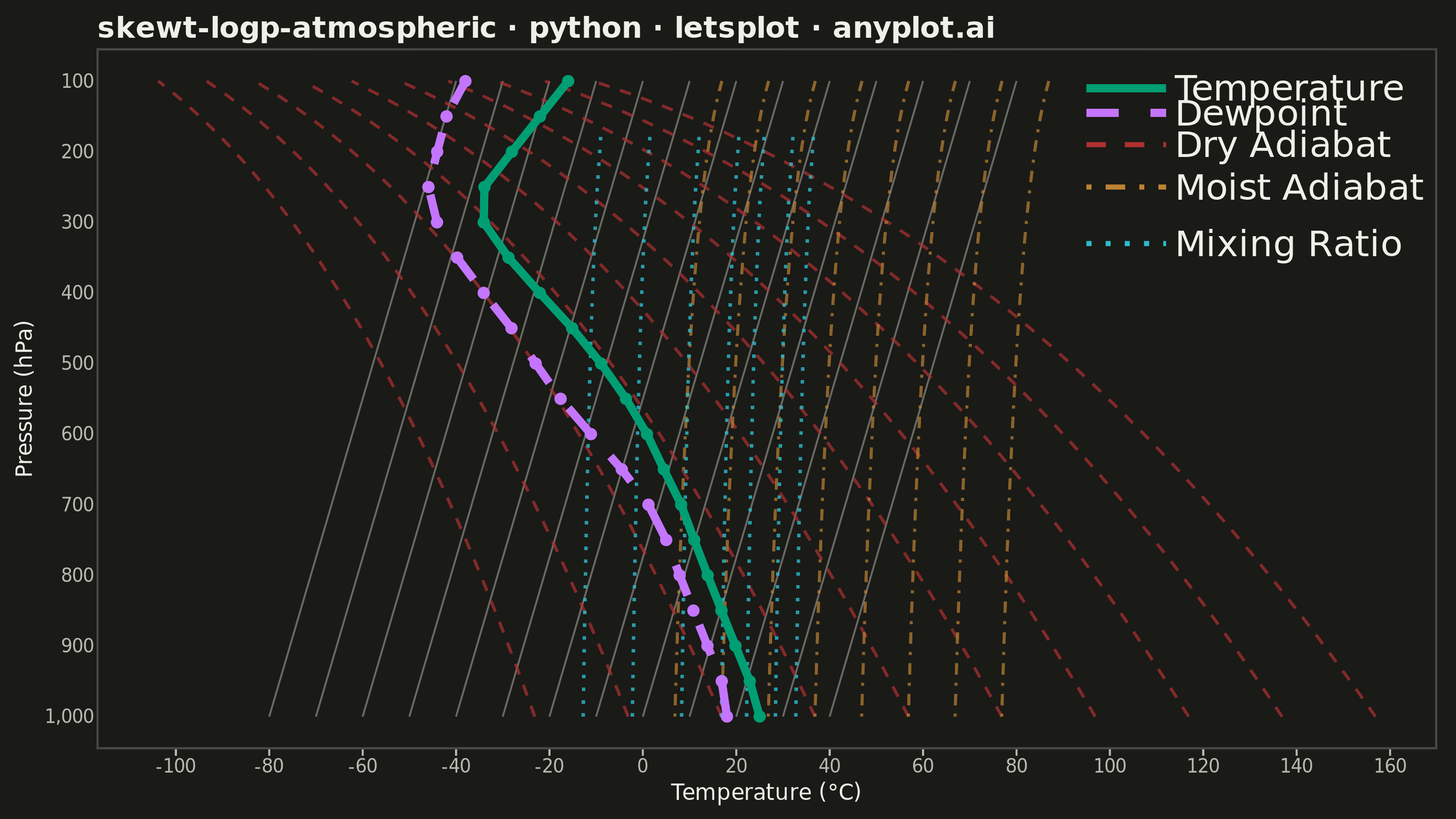
A Skew-T Log-P diagram is a specialized thermodynamic chart used in meteorology to display vertical atmospheric profiles. It features a logarithmic pressure axis (inverted, with surface at bottom) and temperature isotherms skewed 45 degrees to the right, allowing simultaneous visualization of temperature, dewpoint, and derived stability parameters. This diagram is essential for analyzing atmospheric soundings and assessing weather conditions.
""" anyplot.ai
skewt-logp-atmospheric: Skew-T Log-P Atmospheric Diagram
Library: letsplot 4.10.1 | Python 3.13.13
Quality: 82/100 | Updated: 2026-05-21
"""

import os

import numpy as np
import pandas as pd
from lets_plot import (
    LetsPlot,
    aes,
    element_blank,
    element_line,
    element_rect,
    element_text,
    geom_path,
    geom_point,
    geom_segment,
    geom_text,
    ggplot,
    ggsave,
    ggsize,
    labs,
    layer_tooltips,
    scale_y_log10,
    scale_y_reverse,
    theme,
)


LetsPlot.setup_html()

# Theme tokens
THEME = os.getenv("ANYPLOT_THEME", "light")
PAGE_BG = "#FAF8F1" if THEME == "light" else "#1A1A17"
ELEVATED_BG = "#FFFDF6" if THEME == "light" else "#242420"
INK = "#1A1A17" if THEME == "light" else "#F0EFE8"
INK_SOFT = "#4A4A44" if THEME == "light" else "#B8B7B0"

# Okabe-Ito palette — positions 1-6 in order
C_TEMP = "#009E73"  # position 1: temperature profile (primary series)
C_DEWPT = "#C475FD"  # position 2: dewpoint profile
C_DRY = "#AE3030"  # position 5: dry adiabats (background reference)
C_MOIST = "#BD8233"  # position 4: moist adiabats (background reference)
C_MIX = "#2ABCCD"  # position 6: mixing ratio lines (background reference)

# Atmospheric sounding data (synthetic radiosonde profile)
np.random.seed(42)

pressure = np.array([1000, 950, 900, 850, 800, 750, 700, 650, 600, 550, 500, 450, 400, 350, 300, 250, 200, 150, 100])
temperature = np.array([25, 22, 18, 14, 10, 6, 2, -3, -8, -14, -21, -29, -38, -47, -55, -58, -56, -55, -56])
dewpoint = np.array([18, 16, 12, 8, 4, 0, -5, -12, -20, -28, -35, -42, -50, -58, -65, -70, -72, -75, -78])

# Skew-T coordinate transformation: x_plot = T + skew_factor * log10(p0/p)
p0 = 1000
skew_factor = 40

log_pressure = np.log10(p0 / pressure)
temp_skewed = temperature + skew_factor * log_pressure
dewpoint_skewed = dewpoint + skew_factor * log_pressure

# Include original values for interactive tooltips
df_temp = pd.DataFrame({"pressure": pressure, "temp": temperature, "value": temp_skewed})
df_dewpoint = pd.DataFrame({"pressure": pressure, "dewpt": dewpoint, "value": dewpoint_skewed})

# Generate isotherms (skewed 45-degree temperature reference lines)
isotherm_temps = np.arange(-80, 50, 10)
p_range = np.array([1000, 100])
isotherm_data = []
for t in isotherm_temps:
    log_p_vals = np.log10(p0 / p_range)
    t_skewed = t + skew_factor * log_p_vals
    isotherm_data.append({"x_start": t_skewed[0], "x_end": t_skewed[1], "y_start": p_range[0], "y_end": p_range[1]})
df_isotherms = pd.DataFrame(isotherm_data)

# Generate dry adiabats (constant potential temperature lines)
dry_adiabat_thetas = np.arange(250, 450, 20)
p_levels = np.linspace(1000, 100, 50)
dry_adiabat_data = []
for theta in dry_adiabat_thetas:
    temps = (theta * (p_levels / p0) ** 0.286) - 273.15
    log_p_vals = np.log10(p0 / p_levels)
    temps_skewed = temps + skew_factor * log_p_vals
    for i in range(len(p_levels)):
        dry_adiabat_data.append({"pressure": p_levels[i], "temp_skewed": temps_skewed[i], "theta": theta})
df_dry_adiabats = pd.DataFrame(dry_adiabat_data)

# Generate moist adiabats (equivalent potential temperature lines)
moist_adiabat_theta_e = np.arange(280, 360, 10)
moist_adiabat_data = []
for theta_e in moist_adiabat_theta_e:
    t_surface = theta_e - 273.15
    for p in p_levels:
        height_factor = np.log(p0 / p) * 2.5
        t_moist = t_surface - 6.5 * height_factor * 0.8
        log_p_val = np.log10(p0 / p)
        t_skewed = t_moist + skew_factor * log_p_val
        moist_adiabat_data.append({"pressure": p, "temp_skewed": t_skewed, "theta_e": theta_e})
df_moist_adiabats = pd.DataFrame(moist_adiabat_data)

# Generate mixing ratio lines (constant water vapor mixing ratio)
mixing_ratios = [1, 2, 4, 7, 10, 15, 20]
mixing_data = []
for ws in mixing_ratios:
    for p in p_levels[::5]:
        t = 35 * np.log10(ws * p / 622) - 20
        log_p_val = np.log10(p0 / p)
        t_skewed = t + skew_factor * log_p_val
        mixing_data.append({"pressure": p, "temp_skewed": t_skewed, "ws": ws})
df_mixing = pd.DataFrame(mixing_data)

# Theme-adaptive chrome
anyplot_theme = theme(
    plot_background=element_rect(fill=PAGE_BG, color=PAGE_BG),
    panel_background=element_rect(fill=PAGE_BG),
    panel_border=element_blank(),
    panel_grid_major=element_blank(),
    panel_grid_minor=element_blank(),
    axis_title=element_text(color=INK, size=12),
    axis_text=element_text(color=INK_SOFT, size=10),
    axis_line=element_line(color=INK_SOFT),
    axis_ticks=element_line(color=INK_SOFT),
    plot_title=element_text(color=INK, size=16, face="bold"),
    legend_background=element_rect(fill=ELEVATED_BG, color=INK_SOFT),
    legend_text=element_text(color=INK_SOFT, size=10),
    legend_title=element_text(color=INK),
    plot_margin=[8, 8, 8, 8],
)

plot = (
    ggplot()
    # Isotherms (gray diagonal reference lines)
    + geom_segment(
        aes(x="x_start", xend="x_end", y="y_start", yend="y_end"),
        data=df_isotherms,
        color=INK_SOFT,
        size=0.4,
        alpha=0.5,
        tooltips="none",
    )
    # Dry adiabats — Okabe-Ito orange dashed
    + geom_path(
        aes(x="temp_skewed", y="pressure", group="theta"),
        data=df_dry_adiabats,
        color=C_DRY,
        size=0.7,
        alpha=0.7,
        linetype="dashed",
        tooltips="none",
    )
    # Moist adiabats — Okabe-Ito reddish purple dotdash
    + geom_path(
        aes(x="temp_skewed", y="pressure", group="theta_e"),
        data=df_moist_adiabats,
        color=C_MOIST,
        size=0.7,
        alpha=0.7,
        linetype="dotdash",
        tooltips="none",
    )
    # Mixing ratio lines — Okabe-Ito sky blue dotted
    + geom_path(
        aes(x="temp_skewed", y="pressure", group="ws"),
        data=df_mixing,
        color=C_MIX,
        size=0.8,
        alpha=0.8,
        linetype="dotted",
        tooltips="none",
    )
    # Temperature profile — Okabe-Ito green solid (primary series, position 1)
    + geom_path(
        aes(x="value", y="pressure"),
        data=df_temp,
        color=C_TEMP,
        size=2.0,
        tooltips=layer_tooltips().line("Temperature: @temp°C").line("Pressure: @pressure hPa"),
    )
    # Dewpoint profile — Okabe-Ito vermillion dashed (secondary series, position 2)
    + geom_path(
        aes(x="value", y="pressure"),
        data=df_dewpoint,
        color=C_DEWPT,
        size=2.0,
        linetype="dashed",
        tooltips=layer_tooltips().line("Dewpoint: @dewpt°C").line("Pressure: @pressure hPa"),
    )
    # Data points on profiles for clarity
    + geom_point(
        aes(x="value", y="pressure"),
        data=df_temp,
        color=C_TEMP,
        size=3.0,
        tooltips=layer_tooltips().line("Temperature: @temp°C").line("Pressure: @pressure hPa"),
    )
    + geom_point(
        aes(x="value", y="pressure"),
        data=df_dewpoint,
        color=C_DEWPT,
        size=3.0,
        tooltips=layer_tooltips().line("Dewpoint: @dewpt°C").line("Pressure: @pressure hPa"),
    )
    # Logarithmic inverted pressure axis
    + scale_y_log10()
    + scale_y_reverse(limits=[1000, 100])
    + labs(x="Temperature (°C)", y="Pressure (hPa)", title="skewt-logp-atmospheric · python · letsplot · anyplot.ai")
    + ggsize(800, 450)
    + anyplot_theme
)

# Manual legend (positioned upper-right in skewed coordinate space)
legend_x_start = 95
legend_x_end = 112
legend_text_x = 114
legend_entries = [
    {"label": "Temperature", "color": C_TEMP, "linetype": "solid", "size": 2.0, "y": 110},
    {"label": "Dewpoint", "color": C_DEWPT, "linetype": "dashed", "size": 2.0, "y": 145},
    {"label": "Dry Adiabat", "color": C_DRY, "linetype": "dashed", "size": 1.2, "y": 190},
    {"label": "Moist Adiabat", "color": C_MOIST, "linetype": "dotdash", "size": 1.2, "y": 250},
    {"label": "Mixing Ratio", "color": C_MIX, "linetype": "dotted", "size": 1.2, "y": 330},
]

for entry in legend_entries:
    plot = plot + geom_segment(
        aes(x="x_start", xend="x_end", y="y", yend="y"),
        data=pd.DataFrame([{"x_start": legend_x_start, "x_end": legend_x_end, "y": entry["y"]}]),
        color=entry["color"],
        size=entry["size"],
        linetype=entry["linetype"],
        tooltips="none",
    )
    plot = plot + geom_text(x=legend_text_x, y=entry["y"], label=entry["label"], color=INK, size=10, hjust=0)

# Save PNG and HTML for both themes
ggsave(plot, f"plot-{THEME}.png", path=".", scale=4)
ggsave(plot, f"plot-{THEME}.html", path=".")
Runnable source as JSON, for any HTTP client: https://api.anyplot.ai/specs/skewt-logp-atmospheric/letsplot/code. Any spec id and library id listed in llms-full.txt fit the same URL shape; every URL below is complete and callable.
{
  "spec_id": "skewt-logp-atmospheric",
  "language": "python",
  "library": "letsplot",
  "page": "https://anyplot.ai/skewt-logp-atmospheric/python/letsplot",
  "hub": "https://anyplot.ai/skewt-logp-atmospheric",
  "code_json": "https://api.anyplot.ai/specs/skewt-logp-atmospheric/letsplot/code",
  "spec_json": "https://api.anyplot.ai/specs/skewt-logp-atmospheric",
  "render_light_png": "https://storage.googleapis.com/anyplot-images/plots/skewt-logp-atmospheric/python/letsplot/plot-light.png",
  "render_dark_png": "https://storage.googleapis.com/anyplot-images/plots/skewt-logp-atmospheric/python/letsplot/plot-dark.png",
  "interactive_light_html": "https://storage.googleapis.com/anyplot-images/plots/skewt-logp-atmospheric/python/letsplot/plot-light.html",
  "interactive_dark_html": "https://storage.googleapis.com/anyplot-images/plots/skewt-logp-atmospheric/python/letsplot/plot-dark.html",
  "quality_score": 82.0,
  "license": "MIT",
  "guide": "https://anyplot.ai/llms.txt"
}
Part of Skew-T Log-P Atmospheric Diagram on anyplot.ai.