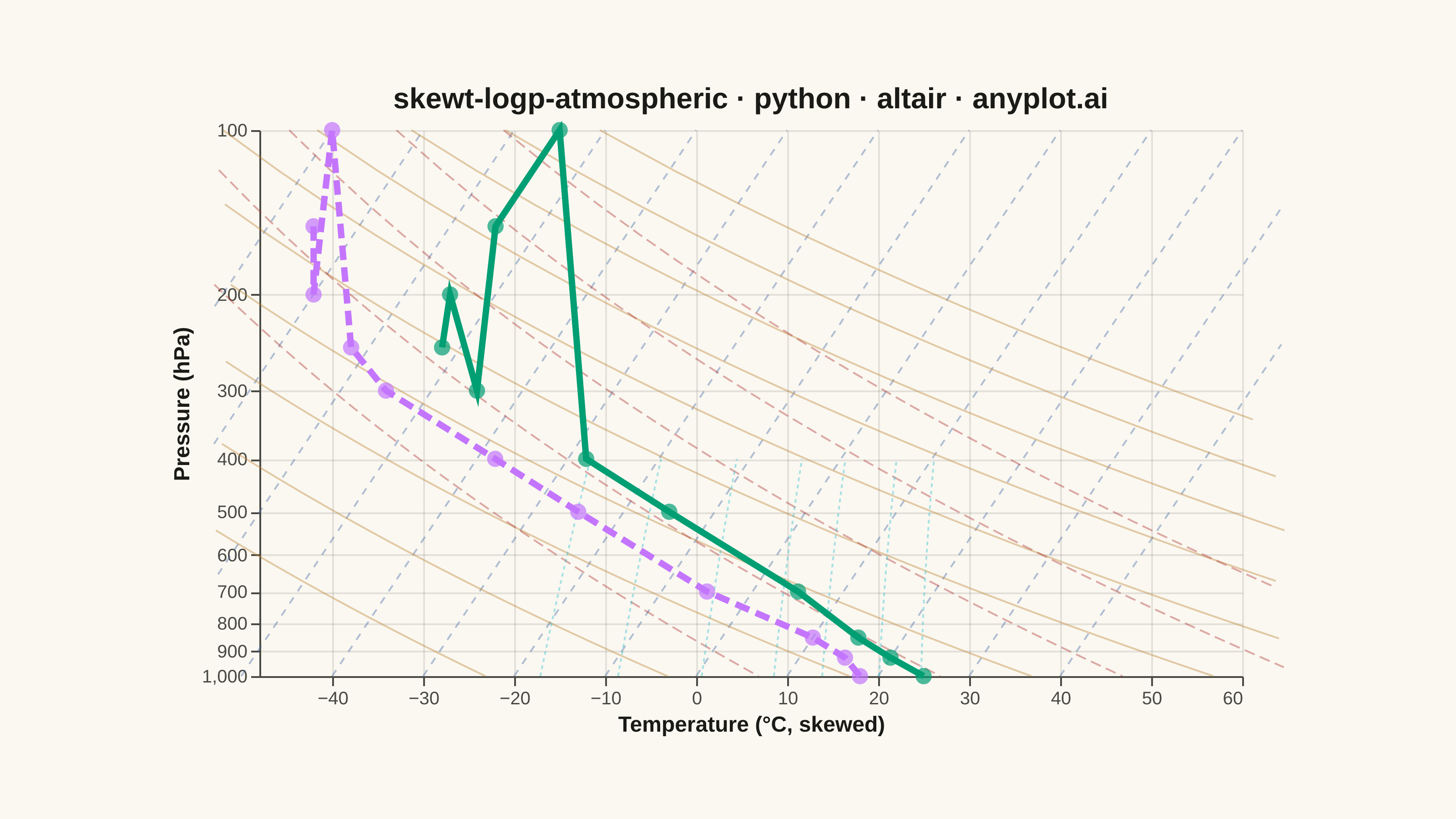
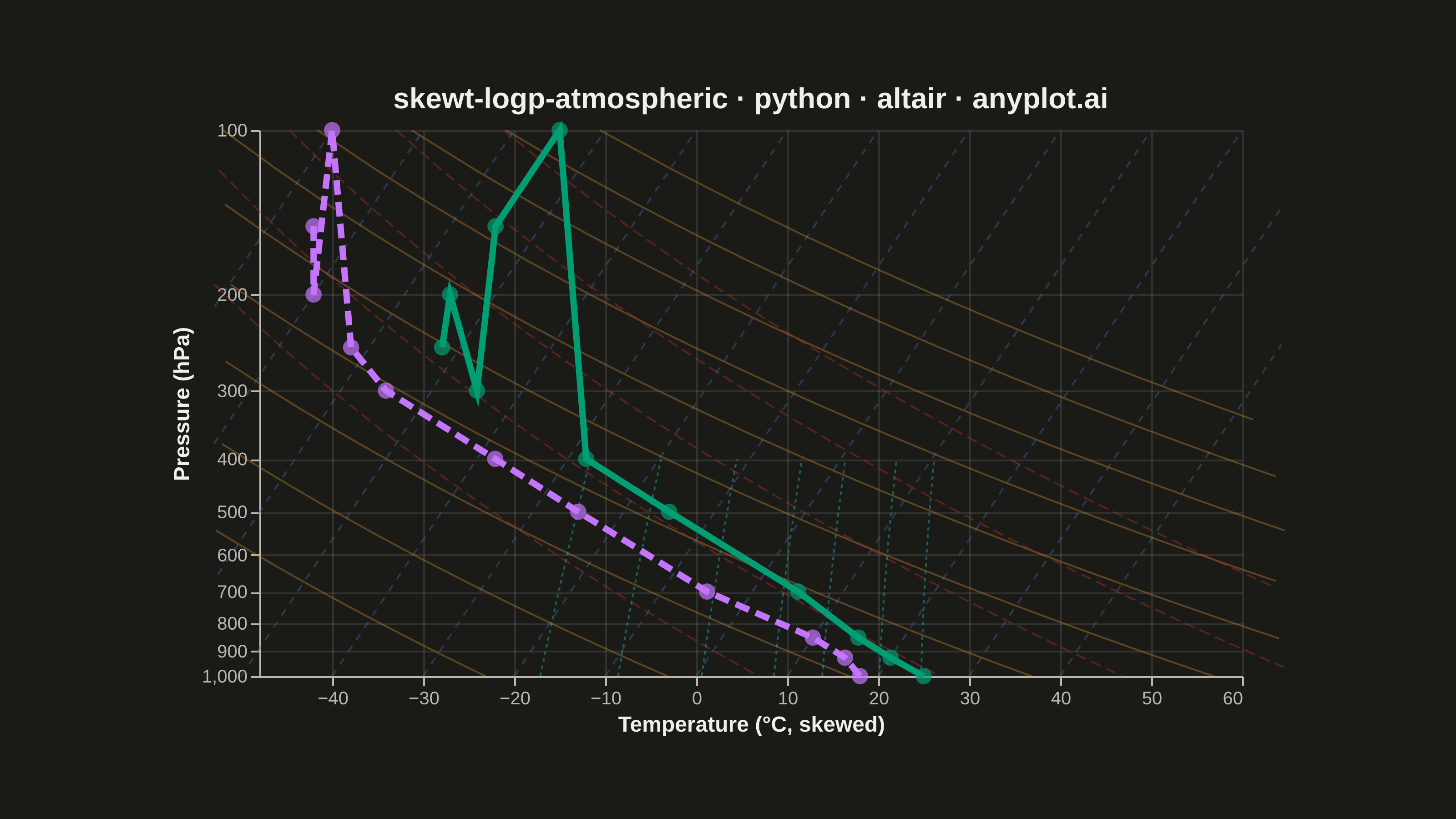
A Skew-T Log-P diagram is a specialized thermodynamic chart used in meteorology to display vertical atmospheric profiles. It features a logarithmic pressure axis (inverted, with surface at bottom) and temperature isotherms skewed 45 degrees to the right, allowing simultaneous visualization of temperature, dewpoint, and derived stability parameters. This diagram is essential for analyzing atmospheric soundings and assessing weather conditions.
""" anyplot.ai
skewt-logp-atmospheric: Skew-T Log-P Atmospheric Diagram
Library: altair 6.1.0 | Python 3.13.13
Quality: 85/100 | Updated: 2026-05-21
"""

import os
import sys


sys.path = sys.path[1:]  # prevent self-import when script is named altair.py

import altair as alt
import numpy as np
import pandas as pd
from PIL import Image


# Theme tokens
THEME = os.getenv("ANYPLOT_THEME", "light")
PAGE_BG = "#FAF8F1" if THEME == "light" else "#1A1A17"
ELEVATED_BG = "#FFFDF6" if THEME == "light" else "#242420"
INK = "#1A1A17" if THEME == "light" else "#F0EFE8"
INK_SOFT = "#4A4A44" if THEME == "light" else "#B8B7B0"

# Data
np.random.seed(42)

pressure = np.array([1000, 925, 850, 700, 500, 400, 300, 250, 200, 150, 100])
temperature = np.array([25, 20, 15, 5, -15, -28, -45, -52, -55, -55, -55])
dewpoint = np.array([18, 15, 10, -5, -25, -38, -55, -62, -70, -75, -80])

skew_factor = 40
log_p_base = np.log10(pressure)
skew_offset = (np.log10(1000) - log_p_base) * skew_factor
temp_skewed = temperature + skew_offset
dew_skewed = dewpoint + skew_offset

# X-axis domain — tightened to reduce whitespace on the right
x_domain = [-48, 60]
X_MARGIN = 5  # pre-filter margin to exclude vl-convert layout inflation from out-of-range values

# Unified color/dash scheme (single legend covers all 6 element types)
# Data series first so Temperature gets Okabe-Ito position 1 (#009E73 brand green)
ALL_LABELS = ["Temperature", "Dewpoint", "Isotherm", "Dry Adiabat", "Moist Adiabat", "Mixing Ratio"]
ALL_COLORS = ["#009E73", "#C475FD", "#4467A3", "#BD8233", "#AE3030", "#2ABCCD"]
ALL_DASHES = [[1, 0], [8, 4], [4, 4], [1, 0], [6, 3], [2, 2]]

full_color_scale = alt.Scale(domain=ALL_LABELS, range=ALL_COLORS)
full_dash_scale = alt.Scale(type="ordinal", domain=ALL_LABELS, range=ALL_DASHES)

# Reference lines — pre-filtered to x_domain ± margin to prevent layout inflation
ref_records = []

for t in np.arange(-80, 50, 10):
    for p_val in np.linspace(100, 1000, 50):
        lp = np.log10(p_val)
        t_sk = t + (np.log10(1000) - lp) * skew_factor
        if x_domain[0] - X_MARGIN <= t_sk <= x_domain[1] + X_MARGIN:
            ref_records.append({"pressure": p_val, "temp_skewed": t_sk, "label": "Isotherm", "line_id": f"iso_{t}"})

for theta in np.arange(250, 450, 20):
    for p_val in np.linspace(100, 1000, 50):
        t_c = theta * (p_val / 1000) ** 0.286 - 273.15
        lp = np.log10(p_val)
        t_sk = t_c + (np.log10(1000) - lp) * skew_factor
        if x_domain[0] - X_MARGIN <= t_sk <= x_domain[1] + X_MARGIN:
            ref_records.append(
                {"pressure": p_val, "temp_skewed": t_sk, "label": "Dry Adiabat", "line_id": f"dry_{theta}"}
            )

for theta_e in np.arange(280, 380, 20):
    for p_val in np.linspace(100, 1000, 50):
        t_c = theta_e * (p_val / 1000) ** 0.23 - 273.15
        lp = np.log10(p_val)
        t_sk = t_c + (np.log10(1000) - lp) * skew_factor
        if x_domain[0] - X_MARGIN <= t_sk <= x_domain[1] + X_MARGIN:
            ref_records.append(
                {"pressure": p_val, "temp_skewed": t_sk, "label": "Moist Adiabat", "line_id": f"moist_{theta_e}"}
            )

for w in [1, 2, 4, 7, 10, 15, 20]:
    for p_val in np.linspace(400, 1000, 30):
        e = (w * p_val) / (622 + w)
        if e > 0.1:
            ln_e = np.log(e / 6.112)
            denom = 17.67 - ln_e
            if denom != 0:
                td = (243.5 * ln_e) / denom
                if -100 < td < 50:
                    lp = np.log10(p_val)
                    t_sk = td + (np.log10(1000) - lp) * skew_factor
                    if x_domain[0] - X_MARGIN <= t_sk <= x_domain[1] + X_MARGIN:
                        ref_records.append(
                            {"pressure": p_val, "temp_skewed": t_sk, "label": "Mixing Ratio", "line_id": f"mix_{w}"}
                        )

ref_df = pd.DataFrame(ref_records)

# Sounding profile data — same 'label' field for unified color/dash scale
prof_records = []
for i in range(len(pressure)):
    prof_records.append({"pressure": pressure[i], "temp_skewed": temp_skewed[i], "label": "Temperature"})
    prof_records.append({"pressure": pressure[i], "temp_skewed": dew_skewed[i], "label": "Dewpoint"})
prof_df = pd.DataFrame(prof_records)

y_scale = alt.Scale(type="log", domain=[1000, 100])

# Reference lines — thin, semi-transparent background grid
ref_lines = (
    alt.Chart(ref_df)
    .mark_line(opacity=0.40, strokeWidth=1.0)
    .encode(
        x=alt.X("temp_skewed:Q", scale=alt.Scale(domain=x_domain), title="Temperature (°C, skewed)"),
        y=alt.Y("pressure:Q", scale=y_scale, title="Pressure (hPa)"),
        detail="line_id:N",
        color=alt.Color("label:N", scale=full_color_scale, legend=None),
        strokeDash=alt.StrokeDash("label:N", scale=full_dash_scale, legend=None),
    )
)

# Sounding profiles — thick lines; legend here shows all 6 labels via shared scale
prof_lines = (
    alt.Chart(prof_df)
    .mark_line(strokeWidth=3.5)
    .encode(
        x=alt.X("temp_skewed:Q", scale=alt.Scale(domain=x_domain)),
        y=alt.Y("pressure:Q", scale=y_scale),
        color=alt.Color(
            "label:N",
            scale=full_color_scale,
            legend=alt.Legend(
                title="", labelFontSize=10, titleFontSize=10, symbolSize=200, symbolStrokeWidth=2, offset=6
            ),
        ),
        strokeDash=alt.StrokeDash("label:N", scale=full_dash_scale, legend=None),
        tooltip=["label:N", "pressure:Q", alt.Tooltip("temp_skewed:Q", title="T skewed (°C)", format=".1f")],
    )
)

# Profile points at each sounding level
prof_points = (
    alt.Chart(prof_df)
    .mark_circle(size=80, filled=True)
    .encode(
        x=alt.X("temp_skewed:Q", scale=alt.Scale(domain=x_domain)),
        y=alt.Y("pressure:Q", scale=y_scale),
        color=alt.Color("label:N", scale=full_color_scale, legend=None),
    )
)

title_text = "skewt-logp-atmospheric · python · altair · anyplot.ai"

# Inner view 540×300 — filtered data keeps total PNG within 3200×1800 after padding
chart = (
    alt.layer(ref_lines, prof_lines, prof_points)
    .resolve_scale(color="shared", strokeDash="shared")
    .properties(
        width=540, height=300, background=PAGE_BG, title=alt.Title(title_text, fontSize=16, color=INK, anchor="middle")
    )
    .configure_view(fill=PAGE_BG, stroke=None)
    .configure_axis(
        domainColor=INK_SOFT,
        tickColor=INK_SOFT,
        gridColor=INK,
        gridOpacity=0.10,
        labelColor=INK_SOFT,
        titleColor=INK,
        labelFontSize=10,
        titleFontSize=12,
    )
    .configure_legend(
        fillColor=ELEVATED_BG,
        strokeColor=INK_SOFT,
        labelColor=INK_SOFT,
        titleColor=INK,
        labelFontSize=10,
        titleFontSize=10,
    )
)

# Save PNG
chart.save(f"plot-{THEME}.png", scale_factor=4.0)

# PAD-only to canonical 3200×1800 — do NOT crop (would clip title/axis labels)
TW, TH = 3200, 1800
_img = Image.open(f"plot-{THEME}.png").convert("RGB")
_w, _h = _img.size
if _w > TW or _h > TH:
    raise SystemExit(
        f"altair vl-convert produced {_w}×{_h}, exceeds target {TW}×{TH}. "
        f"Shrink chart .properties(width=, height=) and re-render."
    )
if _w < TW or _h < TH:
    _canvas = Image.new("RGB", (TW, TH), PAGE_BG)
    _canvas.paste(_img, ((TW - _w) // 2, (TH - _h) // 2))
    _canvas.save(f"plot-{THEME}.png")

# Save HTML
chart.save(f"plot-{THEME}.html")
Runnable source as JSON, for any HTTP client: https://api.anyplot.ai/specs/skewt-logp-atmospheric/altair/code. Any spec id and library id listed in llms-full.txt fit the same URL shape; every URL below is complete and callable.
{
  "spec_id": "skewt-logp-atmospheric",
  "language": "python",
  "library": "altair",
  "page": "https://anyplot.ai/skewt-logp-atmospheric/python/altair",
  "hub": "https://anyplot.ai/skewt-logp-atmospheric",
  "code_json": "https://api.anyplot.ai/specs/skewt-logp-atmospheric/altair/code",
  "spec_json": "https://api.anyplot.ai/specs/skewt-logp-atmospheric",
  "render_light_png": "https://storage.googleapis.com/anyplot-images/plots/skewt-logp-atmospheric/python/altair/plot-light.png",
  "render_dark_png": "https://storage.googleapis.com/anyplot-images/plots/skewt-logp-atmospheric/python/altair/plot-dark.png",
  "interactive_light_html": "https://storage.googleapis.com/anyplot-images/plots/skewt-logp-atmospheric/python/altair/plot-light.html",
  "interactive_dark_html": "https://storage.googleapis.com/anyplot-images/plots/skewt-logp-atmospheric/python/altair/plot-dark.html",
  "quality_score": 85.0,
  "license": "MIT",
  "guide": "https://anyplot.ai/llms.txt"
}
Part of Skew-T Log-P Atmospheric Diagram on anyplot.ai.