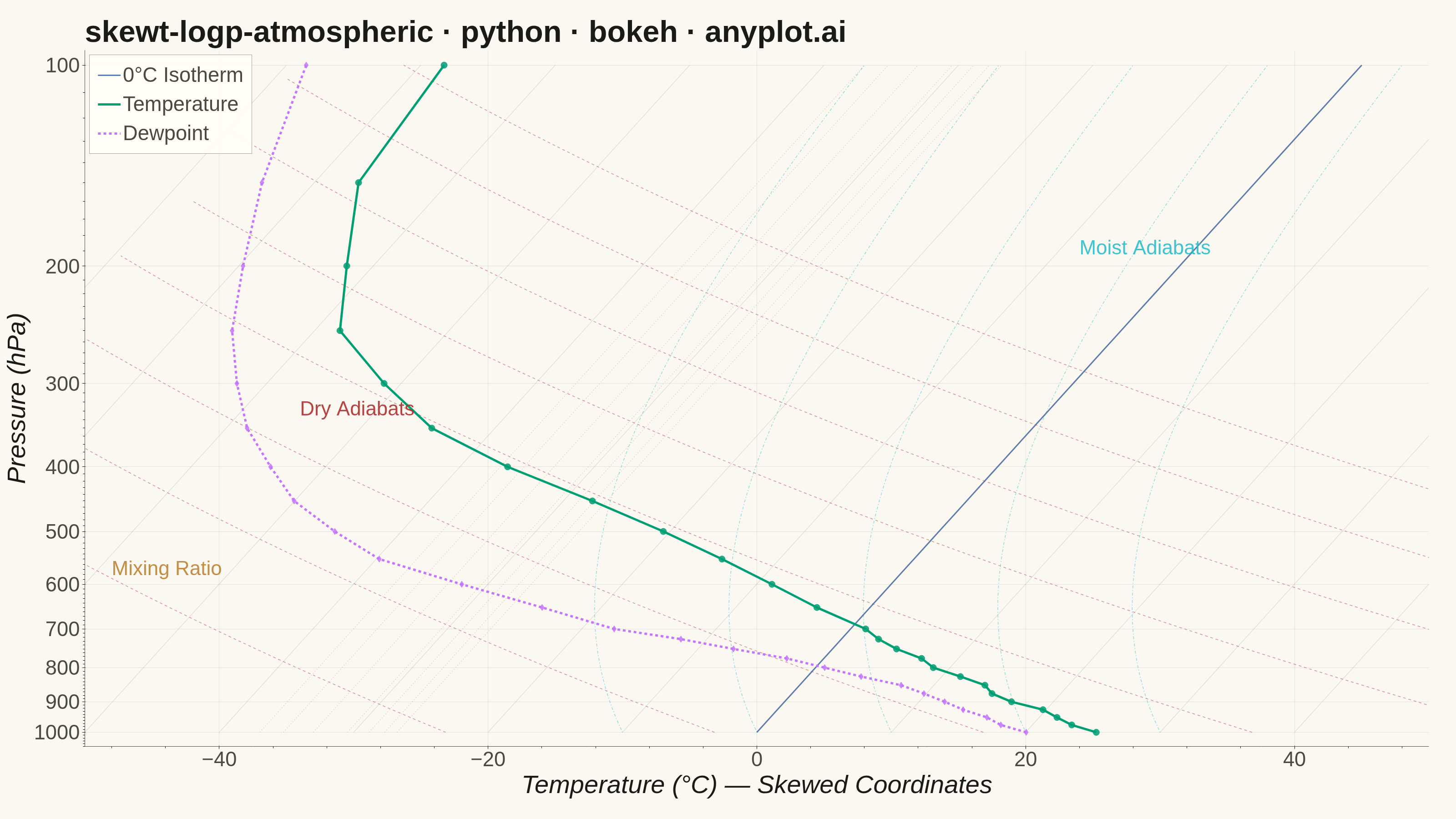
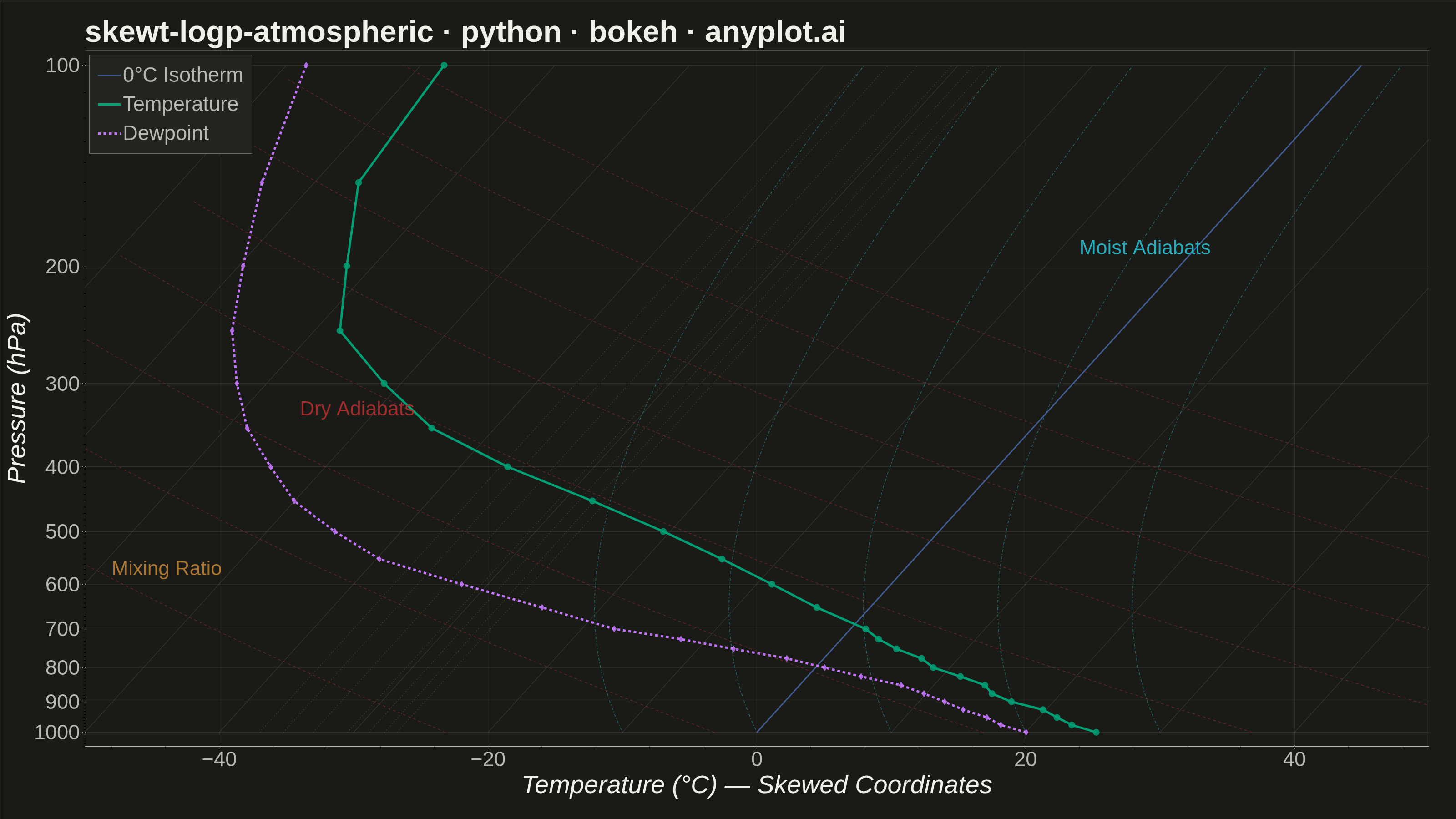
A Skew-T Log-P diagram is a specialized thermodynamic chart used in meteorology to display vertical atmospheric profiles. It features a logarithmic pressure axis (inverted, with surface at bottom) and temperature isotherms skewed 45 degrees to the right, allowing simultaneous visualization of temperature, dewpoint, and derived stability parameters. This diagram is essential for analyzing atmospheric soundings and assessing weather conditions.
""" anyplot.ai
skewt-logp-atmospheric: Skew-T Log-P Atmospheric Diagram
Library: bokeh 3.9.0 | Python 3.13.13
Quality: 87/100 | Updated: 2026-05-21
"""

import os
import time
from pathlib import Path

import numpy as np
from bokeh.io import output_file, save
from bokeh.models import ColumnDataSource, CrosshairTool, HoverTool, Label, WheelZoomTool
from bokeh.plotting import figure
from selenium import webdriver
from selenium.webdriver.chrome.options import Options


# Theme tokens
THEME = os.getenv("ANYPLOT_THEME", "light")
PAGE_BG = "#FAF8F1" if THEME == "light" else "#1A1A17"
ELEVATED_BG = "#FFFDF6" if THEME == "light" else "#242420"
INK = "#1A1A17" if THEME == "light" else "#F0EFE8"
INK_SOFT = "#4A4A44" if THEME == "light" else "#B8B7B0"
INK_MUTED = "#6B6A63" if THEME == "light" else "#A8A79F"

IMPRINT = ["#009E73", "#C475FD", "#4467A3", "#BD8233", "#AE3030", "#2ABCCD", "#954477"]

# Data
np.random.seed(42)

pressure = np.array(
    [
        1000,
        975,
        950,
        925,
        900,
        875,
        850,
        825,
        800,
        775,
        750,
        725,
        700,
        650,
        600,
        550,
        500,
        450,
        400,
        350,
        300,
        250,
        200,
        150,
        100,
    ]
)

temperature = (
    np.array([25, 23, 21, 19, 17, 15, 13, 11, 9, 7, 5, 3, 1, -3, -8, -14, -20, -28, -36, -44, -52, -58, -62, -66, -68])
    + np.random.randn(25) * 0.5
)

dewpoint = (
    np.array(
        [20, 18, 16, 14, 12, 10, 7, 4, 1, -3, -7, -12, -17, -24, -32, -40, -45, -50, -54, -58, -62, -66, -70, -74, -78]
    )
    + np.random.randn(25) * 0.3
)
dewpoint = np.minimum(dewpoint, temperature - 0.5)

SKEW_FACTOR = 45
p_range = np.logspace(np.log10(1000), np.log10(100), 50)

# Skew-transform sounding coordinates
log_p_sounding = np.log10(pressure / 1000.0)
x_temp = temperature - SKEW_FACTOR * log_p_sounding
x_dewpoint = dewpoint - SKEW_FACTOR * log_p_sounding

# Plot
fig = figure(
    width=3200,
    height=1800,
    title="skewt-logp-atmospheric · python · bokeh · anyplot.ai",
    x_axis_label="Temperature (°C) — Skewed Coordinates",
    y_axis_label="Pressure (hPa)",
    y_axis_type="log",
    y_range=(1050, 95),
    x_range=(-50, 50),
    toolbar_location=None,
    min_border_bottom=160,
    min_border_left=180,
    min_border_top=110,
    min_border_right=60,
)

# Theme-adaptive chrome
fig.background_fill_color = PAGE_BG
fig.border_fill_color = PAGE_BG
fig.outline_line_color = None

fig.title.text_color = INK
fig.title.text_font_size = "50pt"
fig.xaxis.axis_label_text_color = INK
fig.yaxis.axis_label_text_color = INK
fig.xaxis.axis_label_text_font_size = "42pt"
fig.yaxis.axis_label_text_font_size = "42pt"
fig.xaxis.major_label_text_color = INK_SOFT
fig.yaxis.major_label_text_color = INK_SOFT
fig.xaxis.major_label_text_font_size = "34pt"
fig.yaxis.major_label_text_font_size = "34pt"
fig.xaxis.axis_line_color = INK_SOFT
fig.yaxis.axis_line_color = INK_SOFT
fig.xaxis.major_tick_line_color = INK_SOFT
fig.yaxis.major_tick_line_color = INK_SOFT
fig.xgrid.grid_line_color = INK
fig.ygrid.grid_line_color = INK
fig.xgrid.grid_line_alpha = 0.10
fig.ygrid.grid_line_alpha = 0.10

# Isotherms (45° skewed background reference lines)
isotherm_temps = np.arange(-80, 50, 10)
for t in isotherm_temps:
    log_p = np.log10(p_range / 1000.0)
    x_iso = np.full_like(p_range, t) - SKEW_FACTOR * log_p
    src = ColumnDataSource(data={"x": x_iso, "y": p_range})
    fig.line(x="x", y="y", source=src, line_color=INK_MUTED, line_width=1.2, line_alpha=0.20)

# Dry adiabats (lines of constant potential temperature)
p0 = 1000.0
kappa = 0.286
for theta in np.arange(250, 400, 20):
    t_adiabat = theta * (p_range / p0) ** kappa - 273.15
    log_p = np.log10(p_range / 1000.0)
    x_adiabat = t_adiabat - SKEW_FACTOR * log_p
    mask = (t_adiabat > -80) & (t_adiabat < 60)
    if np.any(mask):
        src = ColumnDataSource(data={"x": x_adiabat[mask], "y": p_range[mask]})
        fig.line(x="x", y="y", source=src, line_color=IMPRINT[4], line_width=1.5, line_alpha=0.50, line_dash="dashed")

# Moist adiabats (pseudoadiabats — simplified iterative approximation)
for t_start in np.arange(-10, 35, 10):
    t_moist = [t_start]
    p_prev, t_prev = 1000.0, t_start
    for p_level in p_range[1:]:
        dt = -0.006 * (p_prev - p_level) * 10 * 0.5
        t_new = t_prev + dt
        t_moist.append(t_new)
        p_prev, t_prev = p_level, t_new
    t_moist = np.array(t_moist)
    log_p = np.log10(p_range / 1000.0)
    x_moist = t_moist - SKEW_FACTOR * log_p
    mask = (t_moist > -80) & (t_moist < 60)
    if np.any(mask):
        src = ColumnDataSource(data={"x": x_moist[mask], "y": p_range[mask]})
        fig.line(
            x="x", y="y", source=src, line_color=IMPRINT[5], line_width=1.5, line_alpha=0.50, line_dash="dotdash"
        )

# Mixing ratio lines
for mr in [1, 2, 4, 8, 12, 16, 20]:
    td_mr = -40 + 10 * np.log10(mr + 1)
    log_p = np.log10(p_range / 1000.0)
    x_mr = np.full_like(p_range, td_mr) - SKEW_FACTOR * log_p
    src = ColumnDataSource(data={"x": x_mr, "y": p_range})
    fig.line(x="x", y="y", source=src, line_color=IMPRINT[3], line_width=1.2, line_alpha=0.40, line_dash="dotted")

# Highlighted 0°C isotherm
log_p_ref = np.log10(p_range / 1000.0)
x_freeze = -SKEW_FACTOR * log_p_ref
src_freeze = ColumnDataSource(data={"x": x_freeze, "y": p_range})
fig.line(
    x="x", y="y", source=src_freeze, line_color=IMPRINT[2], line_width=3, line_alpha=0.85, legend_label="0°C Isotherm"
)

# Temperature profile
src_temp = ColumnDataSource(data={"x": x_temp, "y": pressure, "temp_c": np.round(temperature, 1)})
fig.line(x="x", y="y", source=src_temp, line_color=IMPRINT[0], line_width=5, legend_label="Temperature")
temp_scatter = fig.scatter(x="x", y="y", source=src_temp, size=14, color=IMPRINT[0], alpha=0.85)

# Dewpoint profile
src_dew = ColumnDataSource(data={"x": x_dewpoint, "y": pressure, "dewpt_c": np.round(dewpoint, 1)})
fig.line(
    x="x", y="y", source=src_dew, line_color=IMPRINT[1], line_width=5, line_dash="dashed", legend_label="Dewpoint"
)
dew_scatter = fig.scatter(x="x", y="y", source=src_dew, size=14, color=IMPRINT[1], alpha=0.85, marker="diamond")

# HoverTools for interactive temperature/pressure display
fig.add_tools(HoverTool(renderers=[temp_scatter], tooltips=[("Pressure", "@y{0} hPa"), ("Temperature", "@temp_c °C")]))
fig.add_tools(HoverTool(renderers=[dew_scatter], tooltips=[("Pressure", "@y{0} hPa"), ("Dewpoint", "@dewpt_c °C")]))
fig.add_tools(CrosshairTool(), WheelZoomTool())

# Reference line labels
fig.add_layout(
    Label(x=-34, y=340, text="Dry Adiabats", text_font_size="33pt", text_color=IMPRINT[4], text_alpha=0.90)
)
fig.add_layout(
    Label(x=24, y=195, text="Moist Adiabats", text_font_size="33pt", text_color=IMPRINT[5], text_alpha=0.90)
)
fig.add_layout(
    Label(x=-48, y=590, text="Mixing Ratio", text_font_size="33pt", text_color=IMPRINT[3], text_alpha=0.90)
)

# Legend
fig.legend.location = "top_left"
fig.legend.label_text_font_size = "34pt"
fig.legend.label_text_color = INK_SOFT
fig.legend.background_fill_color = ELEVATED_BG
fig.legend.border_line_color = INK_SOFT
fig.legend.glyph_height = 50
fig.legend.glyph_width = 50
fig.legend.spacing = 12
fig.legend.padding = 18

# Save interactive HTML
output_file(f"plot-{THEME}.html")
save(fig)

# Screenshot with headless Chrome (Selenium 4 / Selenium Manager)
W, H = 3200, 1800
opts = Options()
for arg in (
    "--headless=new",
    "--no-sandbox",
    "--disable-dev-shm-usage",
    "--disable-gpu",
    f"--window-size={W},{H}",
    "--hide-scrollbars",
):
    opts.add_argument(arg)
driver = webdriver.Chrome(options=opts)
# Override emulated viewport to exactly W×H regardless of browser chrome overhead
driver.execute_cdp_cmd(
    "Emulation.setDeviceMetricsOverride", {"width": W, "height": H, "deviceScaleFactor": 1, "mobile": False}
)
driver.get(f"file://{Path(f'plot-{THEME}.html').resolve()}")
time.sleep(3)
driver.save_screenshot(f"plot-{THEME}.png")
driver.quit()
Runnable source as JSON, for any HTTP client: https://api.anyplot.ai/specs/skewt-logp-atmospheric/bokeh/code. Any spec id and library id listed in llms-full.txt fit the same URL shape; every URL below is complete and callable.
{
  "spec_id": "skewt-logp-atmospheric",
  "language": "python",
  "library": "bokeh",
  "page": "https://anyplot.ai/skewt-logp-atmospheric/python/bokeh",
  "hub": "https://anyplot.ai/skewt-logp-atmospheric",
  "code_json": "https://api.anyplot.ai/specs/skewt-logp-atmospheric/bokeh/code",
  "spec_json": "https://api.anyplot.ai/specs/skewt-logp-atmospheric",
  "render_light_png": "https://storage.googleapis.com/anyplot-images/plots/skewt-logp-atmospheric/python/bokeh/plot-light.png",
  "render_dark_png": "https://storage.googleapis.com/anyplot-images/plots/skewt-logp-atmospheric/python/bokeh/plot-dark.png",
  "interactive_light_html": "https://storage.googleapis.com/anyplot-images/plots/skewt-logp-atmospheric/python/bokeh/plot-light.html",
  "interactive_dark_html": "https://storage.googleapis.com/anyplot-images/plots/skewt-logp-atmospheric/python/bokeh/plot-dark.html",
  "quality_score": 87.0,
  "license": "MIT",
  "guide": "https://anyplot.ai/llms.txt"
}
Part of Skew-T Log-P Atmospheric Diagram on anyplot.ai.