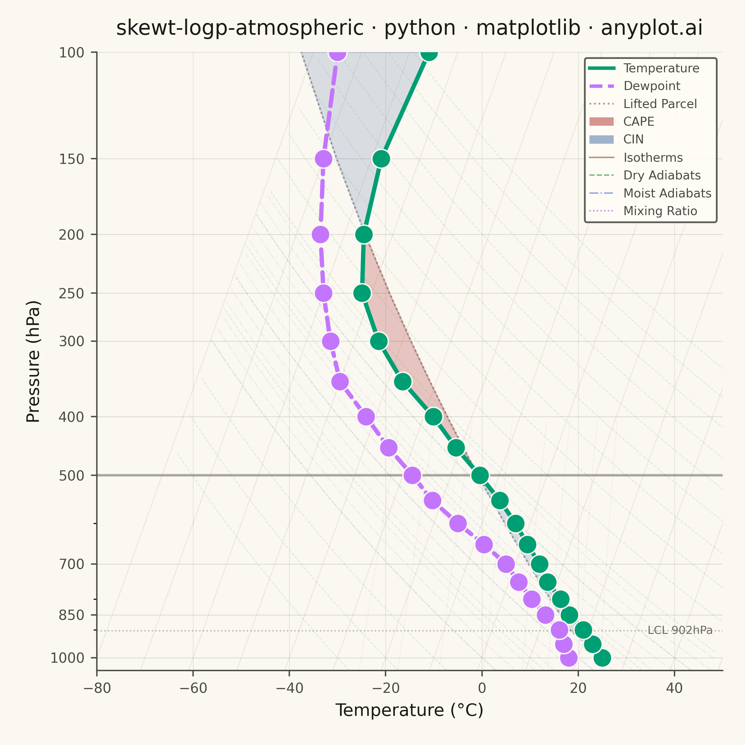
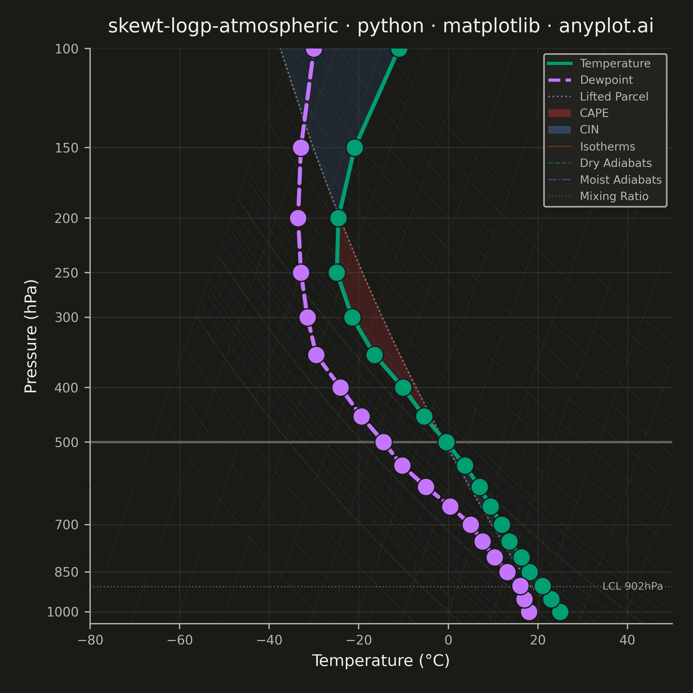
A Skew-T Log-P diagram is a specialized thermodynamic chart used in meteorology to display vertical atmospheric profiles. It features a logarithmic pressure axis (inverted, with surface at bottom) and temperature isotherms skewed 45 degrees to the right, allowing simultaneous visualization of temperature, dewpoint, and derived stability parameters. This diagram is essential for analyzing atmospheric soundings and assessing weather conditions.
""" anyplot.ai
skewt-logp-atmospheric: Skew-T Log-P Atmospheric Diagram
Library: matplotlib 3.10.9 | Python 3.13.13
Quality: 87/100 | Updated: 2026-05-21
"""

import os

import matplotlib.pyplot as plt
import numpy as np
from matplotlib.lines import Line2D
from matplotlib.patches import Patch
from matplotlib.ticker import ScalarFormatter


# Theme tokens
THEME = os.getenv("ANYPLOT_THEME", "light")
PAGE_BG = "#FAF8F1" if THEME == "light" else "#1A1A17"
ELEVATED_BG = "#FFFDF6" if THEME == "light" else "#242420"
INK = "#1A1A17" if THEME == "light" else "#F0EFE8"
INK_SOFT = "#4A4A44" if THEME == "light" else "#B8B7B0"
INK_MUTED = "#6B6A63" if THEME == "light" else "#A8A79F"
# Boost reference line visibility on dark background
REF_ALPHA = 0.10 if THEME == "light" else 0.18

# Okabe-Ito — data series
TEMP_COLOR = "#009E73"  # temperature — position 1
DEWPOINT_COLOR = "#C475FD"  # dewpoint — position 2
CAPE_COLOR = "#AE3030"  # CAPE shading — position 5
CIN_COLOR = "#4467A3"  # CIN shading — position 3

# Data — simulated mid-latitude radiosonde sounding (surface to upper troposphere)
np.random.seed(42)
pressure = np.array([1000, 950, 900, 850, 800, 750, 700, 650, 600, 550, 500, 450, 400, 350, 300, 250, 200, 150, 100])
temperature = np.array([25, 22, 19, 15, 12, 8, 5, 1, -3, -8, -14, -21, -28, -37, -45, -52, -56, -58, -56])
dewpoint = np.array([18, 16, 14, 10, 6, 2, -2, -8, -15, -22, -28, -35, -42, -50, -55, -60, -65, -70, -75])

# Lifted parcel — Bolton (1980) LCL + simplified moist adiabat above for CAPE/CIN shading
T0_K = temperature[0] + 273.15
Td0_K = dewpoint[0] + 273.15
P0 = float(pressure[0])
T_lcl_K = 1.0 / (1.0 / (Td0_K - 56.0) + np.log(T0_K / Td0_K) / 800.0) + 56.0
P_lcl = P0 * (T_lcl_K / T0_K) ** 3.5  # ~902 hPa
parcel_temp = np.where(
    pressure > P_lcl,
    T0_K * (pressure / P0) ** 0.286 - 273.15,  # dry adiabatic below LCL
    T_lcl_K * (pressure / P_lcl) ** 0.19 - 273.15,  # moist adiabatic above LCL
)

# Plot — square canvas for symmetric atmospheric profile
fig, ax = plt.subplots(figsize=(6, 6), dpi=400, facecolor=PAGE_BG)
ax.set_facecolor(PAGE_BG)

ax.set_yscale("log")
ax.set_ylim(1050, 100)
ax.set_xlim(-80, 50)

ax.yaxis.set_major_formatter(ScalarFormatter())
ax.set_yticks([1000, 850, 700, 500, 400, 300, 250, 200, 150, 100])

# Precompute skew offsets (45-degree skew of temperature axis)
p0_ref = 1000.0
p_range = np.logspace(np.log10(1050), np.log10(100), 100)
skew_ref = 45.0 * (np.log(p_range) - np.log(p0_ref)) / (np.log(100) - np.log(p0_ref))
skew_data = 45.0 * (np.log(pressure) - np.log(p0_ref)) / (np.log(100) - np.log(p0_ref))

# Reference lines — isotherms (constant temperature, skewed 45°)
for t in np.arange(-80, 60, 10):
    ax.plot(t + skew_ref, p_range, color="#8B4513", alpha=REF_ALPHA, linewidth=0.5)

# Dry adiabats (constant potential temperature)
for theta in np.arange(-30, 150, 10):
    t_dry = (theta + 273.15) * (p_range / 1000) ** 0.286 - 273.15
    mask = (t_dry > -80) & (t_dry < 50)
    if np.any(mask):
        ax.plot(
            t_dry[mask] + skew_ref[mask],
            p_range[mask],
            color="#228B22",
            alpha=REF_ALPHA * 1.3,
            linewidth=0.5,
            linestyle="--",
        )

# Moist adiabats (simplified saturated-adiabatic lapse rate)
for theta_e in np.arange(0, 50, 4):
    t_dry = (theta_e + 273.15) * (p_range / 1000) ** 0.286 - 273.15
    moisture_factor = np.clip((t_dry + 30) / 60, 0, 1) * 0.5
    t_moist = t_dry * (1 - moisture_factor * (1 - (p_range / 1000) ** 0.2))
    mask = (t_moist > -80) & (t_moist < 50)
    if np.any(mask):
        ax.plot(
            t_moist[mask] + skew_ref[mask],
            p_range[mask],
            color="#4169E1",
            alpha=REF_ALPHA * 1.1,
            linewidth=0.5,
            linestyle="-.",
        )

# Mixing ratio lines (constant water vapor mixing ratio)
for w in [0.5, 1, 2, 4, 7, 10, 15, 20]:
    e = (w * p_range) / (622 + w)
    td = 243.5 * np.log(e / 6.112) / (17.67 - np.log(e / 6.112))
    mask = (td > -80) & (td < 50) & (p_range >= 400)
    if np.any(mask):
        ax.plot(
            td[mask] + skew_ref[mask],
            p_range[mask],
            color="#9932CC",
            alpha=REF_ALPHA * 1.3,
            linewidth=0.5,
            linestyle=":",
        )

# Skewed coordinates for profiles
temp_skewed = temperature + skew_data
dewpoint_skewed = dewpoint + skew_data
parcel_skewed = parcel_temp + skew_data

# CAPE/CIN shading — meteorological insight into convective potential
ax.fill_betweenx(
    pressure,
    temp_skewed,
    parcel_skewed,
    where=(parcel_temp < temperature),
    alpha=0.18,
    color=CIN_COLOR,
    zorder=2,
    interpolate=True,
)
ax.fill_betweenx(
    pressure,
    temp_skewed,
    parcel_skewed,
    where=(parcel_temp >= temperature),
    alpha=0.25,
    color=CAPE_COLOR,
    zorder=2,
    interpolate=True,
)

# Lifted parcel trace
ax.plot(parcel_skewed, pressure, color=INK_MUTED, linewidth=1.0, linestyle=":", zorder=3.5, alpha=0.65)

# 500 hPa emphasis — key synoptic reference level
ax.axhline(y=500, color=INK_SOFT, linewidth=1.5, alpha=0.4, linestyle="-", zorder=1.5)

# Data profiles
ax.plot(temp_skewed, pressure, color=TEMP_COLOR, linewidth=2.5, solid_capstyle="round", zorder=4)
ax.scatter(temp_skewed, pressure, color=TEMP_COLOR, s=120, zorder=5, edgecolors=PAGE_BG, linewidth=0.8)

ax.plot(dewpoint_skewed, pressure, color=DEWPOINT_COLOR, linewidth=2.5, linestyle="--", dash_capstyle="round", zorder=4)
ax.scatter(dewpoint_skewed, pressure, color=DEWPOINT_COLOR, s=120, zorder=5, edgecolors=PAGE_BG, linewidth=0.8)

# LCL annotation — lifted condensation level (base of cumulus clouds)
ax.axhline(y=P_lcl, color=INK_MUTED, linewidth=0.8, alpha=0.45, linestyle=":", zorder=3)
ax.text(48, P_lcl, f"LCL {P_lcl:.0f}hPa", fontsize=6.5, color=INK_MUTED, va="center", ha="right")

# Style
ax.set_xlabel("Temperature (°C)", fontsize=10, color=INK)
ax.set_ylabel("Pressure (hPa)", fontsize=10, color=INK)
ax.set_title(
    "skewt-logp-atmospheric · python · matplotlib · anyplot.ai", fontsize=12, fontweight="medium", color=INK, pad=10
)
ax.tick_params(axis="both", labelsize=8, colors=INK_SOFT, labelcolor=INK_SOFT)
ax.spines["top"].set_visible(False)
ax.spines["right"].set_visible(False)
for spine in ("left", "bottom"):
    ax.spines[spine].set_color(INK_SOFT)

ax.yaxis.grid(True, alpha=0.12, linewidth=0.5, color=INK)
ax.xaxis.grid(True, alpha=0.08, linewidth=0.5, color=INK)

# Legend
legend_elements = [
    Line2D([0], [0], color=TEMP_COLOR, linewidth=2, label="Temperature"),
    Line2D([0], [0], color=DEWPOINT_COLOR, linewidth=2, linestyle="--", label="Dewpoint"),
    Line2D([0], [0], color=INK_MUTED, linewidth=1, linestyle=":", alpha=0.65, label="Lifted Parcel"),
    Patch(facecolor=CAPE_COLOR, alpha=0.5, label="CAPE"),
    Patch(facecolor=CIN_COLOR, alpha=0.5, label="CIN"),
    Line2D([0], [0], color="#8B4513", linewidth=0.8, alpha=0.6, label="Isotherms"),
    Line2D([0], [0], color="#228B22", linewidth=0.8, alpha=0.6, linestyle="--", label="Dry Adiabats"),
    Line2D([0], [0], color="#4169E1", linewidth=0.8, alpha=0.6, linestyle="-.", label="Moist Adiabats"),
    Line2D([0], [0], color="#9932CC", linewidth=0.8, alpha=0.6, linestyle=":", label="Mixing Ratio"),
]
leg = ax.legend(handles=legend_elements, loc="upper right", fontsize=7, framealpha=0.9)
leg.get_frame().set_facecolor(ELEVATED_BG)
leg.get_frame().set_edgecolor(INK_SOFT)
plt.setp(leg.get_texts(), color=INK_SOFT)

fig.subplots_adjust(left=0.13, right=0.97, top=0.93, bottom=0.10)

# Save
plt.savefig(f"plot-{THEME}.png", dpi=400, facecolor=PAGE_BG)
Runnable source as JSON, for any HTTP client: https://api.anyplot.ai/specs/skewt-logp-atmospheric/matplotlib/code. Any spec id and library id listed in llms-full.txt fit the same URL shape; every URL below is complete and callable.
{
  "spec_id": "skewt-logp-atmospheric",
  "language": "python",
  "library": "matplotlib",
  "page": "https://anyplot.ai/skewt-logp-atmospheric/python/matplotlib",
  "hub": "https://anyplot.ai/skewt-logp-atmospheric",
  "code_json": "https://api.anyplot.ai/specs/skewt-logp-atmospheric/matplotlib/code",
  "spec_json": "https://api.anyplot.ai/specs/skewt-logp-atmospheric",
  "render_light_png": "https://storage.googleapis.com/anyplot-images/plots/skewt-logp-atmospheric/python/matplotlib/plot-light.png",
  "render_dark_png": "https://storage.googleapis.com/anyplot-images/plots/skewt-logp-atmospheric/python/matplotlib/plot-dark.png",
  "quality_score": 87.0,
  "license": "MIT",
  "guide": "https://anyplot.ai/llms.txt"
}
Part of Skew-T Log-P Atmospheric Diagram on anyplot.ai.