The same plot in 14 other libraries — JavaScript: D3.js, Apache ECharts, Highcharts, MUI X Charts; Python: Altair, Bokeh, lets-plot, Matplotlib, Plotly, plotnine, Pygal, Seaborn; R: ggplot2; Julia: Makie.jl. Compare all 15 side by side: Skew-T Log-P Atmospheric Diagram in Python, R, Julia and JavaScript.
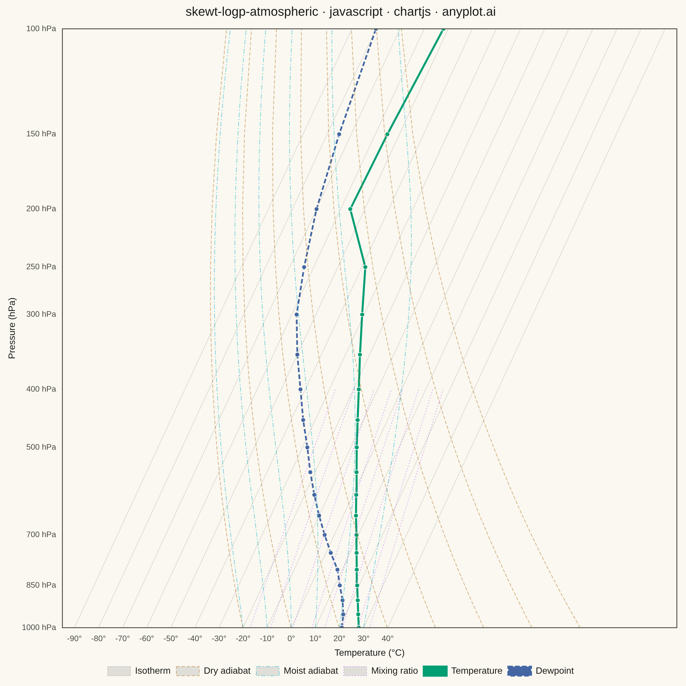
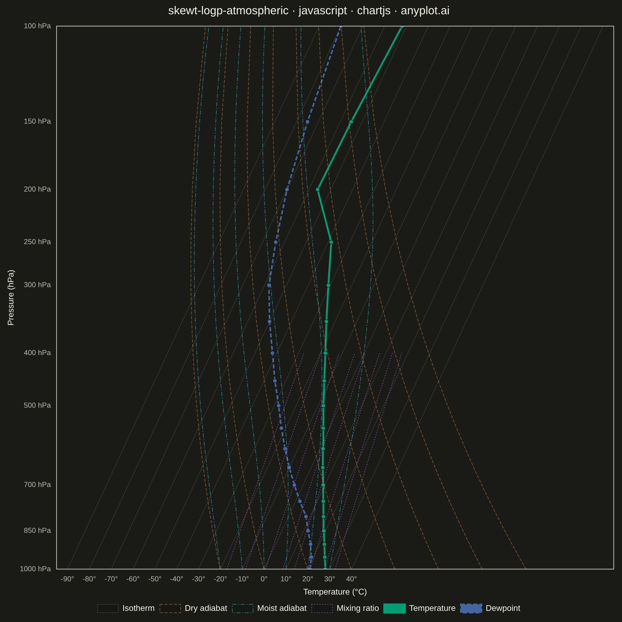
A Skew-T Log-P diagram is a specialized thermodynamic chart used in meteorology to display vertical atmospheric profiles. It features a logarithmic pressure axis (inverted, with surface at bottom) and temperature isotherms skewed 45 degrees to the right, allowing simultaneous visualization of temperature, dewpoint, and derived stability parameters. This diagram is essential for analyzing atmospheric soundings and assessing weather conditions.
// anyplot.ai
// skewt-logp-atmospheric: Skew-T Log-P Atmospheric Diagram
// Library: chartjs 4.4.7 | JavaScript 22.23.2
// Quality: 93/100 | Created: 2026-08-26
//# anyplot-orientation: square

const t = window.ANYPLOT_TOKENS;

const withAlpha = (hex, alpha) => {
  const r = parseInt(hex.slice(1, 3), 16);
  const g = parseInt(hex.slice(3, 5), 16);
  const b = parseInt(hex.slice(5, 7), 16);
  return `rgba(${r}, ${g}, ${b}, ${alpha})`;
};

// --- Skew-T log-P transform --------------------------------------------------
// y is log-pressure (inverted so 1000 hPa sits at the bottom); x is temperature
// skewed to the right by an amount proportional to ln(P0/P), so isotherms
// render as ~45 deg diagonals instead of verticals while the x-axis ticks still
// read as plain surface-level degrees Celsius (the classic skew-T convention).
const P0 = 1000;
const SKEW = 50;
const yOf = (pressureHpa) => -Math.log(pressureHpa);
const skewedX = (tempC, pressureHpa) => tempC + SKEW * Math.log(P0 / pressureHpa);

const P_BOTTOM = 1000;
const P_TOP = 100;
const Y_BOTTOM = yOf(P_BOTTOM);
const Y_TOP = yOf(P_TOP);
const X_MIN = -95;
const X_MAX = 160;

// --- Sounding data (synthetic mid-latitude summer afternoon profile) --------
const pressures = [1000, 950, 900, 850, 800, 750, 700, 650, 600, 550, 500, 450, 400, 350, 300, 250, 200, 150, 100];
const temperature = [28, 25.2, 22.3, 19.2, 16, 12.7, 9.2, 5.3, 1.4, -2.8, -7.5, -12.4, -17.8, -24, -30.8, -38.6, -56, -55, -52];
const dewpoint = [21, 19, 16, 12, 8, 2, -4, -10, -16, -22, -28, -35, -42, -50, -58, -64, -70, -75, -80];

// --- Reference lines ---------------------------------------------------------
// Isotherms: straight diagonals at constant temperature.
const isothermValues = [];
for (let temp = -90; temp <= 40; temp += 10) isothermValues.push(temp);
const isothermDatasets = isothermValues.map((temp, i) => ({
  label: i === 0 ? "Isotherm" : "",
  data: [
    { x: skewedX(temp, P_BOTTOM), y: Y_BOTTOM },
    { x: skewedX(temp, P_TOP), y: Y_TOP },
  ],
  showLine: true,
  borderColor: t.grid,
  borderWidth: 1,
  pointRadius: 0,
  tension: 0,
}));

// Dry adiabats: constant potential temperature, T(P) = theta*(P/P0)^(Rd/Cpd) - 273.15.
const RD_OVER_CPD = 0.2854;
const dryAdiabatThetas = [253, 273, 293, 313, 333, 353, 373, 393]; // Kelvin
const dryAdiabatDatasets = dryAdiabatThetas.map((theta, i) => {
  const points = [];
  for (let p = P_BOTTOM; p >= P_TOP - 1; p -= 50) {
    const temp = theta * Math.pow(p / P0, RD_OVER_CPD) - 273.15;
    points.push({ x: skewedX(temp, p), y: yOf(p) });
  }
  return {
    label: i === 0 ? "Dry adiabat" : "",
    data: points,
    showLine: true,
    borderColor: withAlpha(t.palette[3], 0.6),
    borderDash: [6, 3],
    borderWidth: 1.25,
    pointRadius: 0,
    tension: 0,
  };
});

// Moist (pseudo-) adiabats: integrate the saturated adiabatic lapse rate
// upward from a surface starting temperature, using Bolton's saturation
// vapor pressure approximation for the mixing ratio term.
const saturationVaporPressure = (tempC) => 6.112 * Math.exp((17.67 * tempC) / (tempC + 243.5));
const saturationMixingRatio = (tempC, pressureHpa) => {
  const es = saturationVaporPressure(tempC);
  return (0.622 * es) / (pressureHpa - es);
};
const moistLapseRate = (tempC, pressureHpa) => {
  const tempK = tempC + 273.15;
  const ws = saturationMixingRatio(tempC, pressureHpa);
  const Lv = 2501000;
  const Rd = 287;
  const Cpd = 1004;
  const epsilon = 0.622;
  const numerator = Rd * tempK + Lv * ws;
  const denominator = Cpd + (Lv * Lv * ws * epsilon) / (Rd * tempK * tempK);
  return numerator / (denominator * pressureHpa); // dT/dP, K per hPa
};
const moistAdiabatStarts = [-20, -10, 0, 10, 20, 30]; // deg C at 1000 hPa
const moistAdiabatDatasets = moistAdiabatStarts.map((startTemp, i) => {
  const points = [{ x: skewedX(startTemp, P_BOTTOM), y: Y_BOTTOM }];
  let temp = startTemp;
  let p = P_BOTTOM;
  const dp = -5;
  while (p > P_TOP) {
    temp += moistLapseRate(temp, p) * dp;
    p += dp;
    points.push({ x: skewedX(temp, p), y: yOf(p) });
  }
  return {
    label: i === 0 ? "Moist adiabat" : "",
    data: points,
    showLine: true,
    borderColor: withAlpha(t.palette[5], 0.6),
    borderDash: [8, 3, 2, 3],
    borderWidth: 1.25,
    pointRadius: 0,
    tension: 0,
  };
});

// Mixing ratio lines: constant saturation mixing ratio, inverting Bolton's
// formula to get the dewpoint that saturates at each pressure level.
const dewpointFromMixingRatio = (mixingRatioGkg, pressureHpa) => {
  const vaporPressure = (mixingRatioGkg * pressureHpa) / (622 + mixingRatioGkg);
  const lnRatio = Math.log(vaporPressure / 6.112);
  return (243.5 * lnRatio) / (17.67 - lnRatio);
};
const mixingRatioValues = [1, 2, 4, 7, 10, 16, 24, 32]; // g/kg
const mixingRatioDatasets = mixingRatioValues.map((ratio, i) => {
  const points = [];
  for (let p = P_BOTTOM; p >= 400; p -= 50) {
    const temp = dewpointFromMixingRatio(ratio, p);
    points.push({ x: skewedX(temp, p), y: yOf(p) });
  }
  return {
    label: i === 0 ? "Mixing ratio" : "",
    data: points,
    showLine: true,
    borderColor: withAlpha(t.palette[1], 0.6),
    borderDash: [2, 3],
    borderWidth: 1.25,
    pointRadius: 0,
    tension: 0,
  };
});

// --- Observed profile (drawn last so it sits above the reference lines) ----
const temperatureDataset = {
  label: "Temperature",
  data: pressures.map((p, i) => ({ x: skewedX(temperature[i], p), y: yOf(p) })),
  showLine: true,
  borderColor: t.palette[0],
  backgroundColor: t.palette[0],
  borderWidth: 3.5,
  pointRadius: 4,
  pointBackgroundColor: t.palette[0],
  pointBorderColor: t.pageBg,
  pointBorderWidth: 1,
  tension: 0,
};
const dewpointDataset = {
  label: "Dewpoint",
  data: pressures.map((p, i) => ({ x: skewedX(dewpoint[i], p), y: yOf(p) })),
  showLine: true,
  borderColor: t.palette[2],
  backgroundColor: t.palette[2],
  borderDash: [8, 4],
  borderWidth: 3,
  pointRadius: 4,
  pointBackgroundColor: t.palette[2],
  pointBorderColor: t.pageBg,
  pointBorderWidth: 1,
  tension: 0,
};

const datasets = [
  ...isothermDatasets,
  ...dryAdiabatDatasets,
  ...moistAdiabatDatasets,
  ...mixingRatioDatasets,
  temperatureDataset,
  dewpointDataset,
];

// --- Tooltip: recover real temperature/pressure from the skewed coordinates -
const realTempAt = (skewedXValue, pressureHpa) => skewedXValue - SKEW * Math.log(P0 / pressureHpa);

// --- Axis ticks: pressure labels + surface-referenced temperature labels ---
const pressureTickValues = [1000, 850, 700, 500, 400, 300, 250, 200, 150, 100];
const temperatureTickValues = [];
for (let temp = -90; temp <= 40; temp += 10) temperatureTickValues.push(temp);

// --- Mount -------------------------------------------------------------------
const canvas = document.createElement("canvas");
document.getElementById("container").appendChild(canvas);

// --- Frame: chart.js only borders the axis edges, so draw the remaining two
// sides of the enclosing rectangle that a Skew-T diagram conventionally has.
const framePlugin = {
  id: "skewtFrame",
  afterDraw(chart) {
    const { ctx, chartArea } = chart;
    ctx.save();
    ctx.strokeStyle = t.inkSoft;
    ctx.lineWidth = 1.5;
    ctx.strokeRect(chartArea.left, chartArea.top, chartArea.right - chartArea.left, chartArea.bottom - chartArea.top);
    ctx.restore();
  },
};

new Chart(canvas, {
  type: "scatter",
  data: { datasets },
  plugins: [framePlugin],
  options: {
    responsive: true,
    maintainAspectRatio: false,
    animation: false,
    layout: { padding: { top: 8, right: 16, bottom: 8, left: 8 } },
    plugins: {
      title: {
        display: true,
        text: "skewt-logp-atmospheric · javascript · chartjs · anyplot.ai",
        color: t.ink,
        font: { size: 22, weight: "500" },
        padding: { bottom: 16 },
      },
      legend: {
        position: "bottom",
        labels: {
          color: t.ink,
          font: { size: 16 },
          filter: (legendItem) => Boolean(legendItem.text),
        },
      },
      tooltip: {
        callbacks: {
          title: () => "",
          label: (ctx) => {
            const pressureHpa = Math.exp(-ctx.parsed.y);
            const tempC = realTempAt(ctx.parsed.x, pressureHpa);
            const name = ctx.dataset.label || "Reference line";
            return `${name}: ${tempC.toFixed(1)}°C @ ${pressureHpa.toFixed(0)} hPa`;
          },
        },
      },
    },
    scales: {
      x: {
        type: "linear",
        min: X_MIN,
        max: X_MAX,
        title: { display: true, text: "Temperature (°C)", color: t.ink, font: { size: 16 } },
        grid: { display: false },
        border: { display: true, color: t.inkSoft },
        afterBuildTicks: (axis) => {
          axis.ticks = temperatureTickValues.map((value) => ({ value }));
        },
        ticks: {
          color: t.inkSoft,
          font: { size: 14 },
          callback: (value) => `${value}°`,
        },
      },
      y: {
        type: "linear",
        min: Y_BOTTOM,
        max: Y_TOP,
        title: { display: true, text: "Pressure (hPa)", color: t.ink, font: { size: 16 } },
        grid: { display: false },
        border: { display: true, color: t.inkSoft },
        afterBuildTicks: (axis) => {
          axis.ticks = pressureTickValues.map((value) => ({ value: yOf(value) }));
        },
        ticks: {
          color: t.inkSoft,
          font: { size: 14 },
          callback: (value) => `${Math.round(Math.exp(-value))} hPa`,
        },
      },
    },
  },
});
Runnable source as JSON, for any HTTP client: https://api.anyplot.ai/specs/skewt-logp-atmospheric/chartjs/code. Any spec id and library id listed in llms-full.txt fit the same URL shape; every URL below is complete and callable.
{
  "spec_id": "skewt-logp-atmospheric",
  "language": "javascript",
  "library": "chartjs",
  "page": "https://anyplot.ai/skewt-logp-atmospheric/javascript/chartjs",
  "hub": "https://anyplot.ai/skewt-logp-atmospheric",
  "code_json": "https://api.anyplot.ai/specs/skewt-logp-atmospheric/chartjs/code",
  "spec_json": "https://api.anyplot.ai/specs/skewt-logp-atmospheric",
  "render_light_png": "https://storage.googleapis.com/anyplot-images/plots/skewt-logp-atmospheric/javascript/chartjs/plot-light.png",
  "render_dark_png": "https://storage.googleapis.com/anyplot-images/plots/skewt-logp-atmospheric/javascript/chartjs/plot-dark.png",
  "interactive_light_html": "https://storage.googleapis.com/anyplot-images/plots/skewt-logp-atmospheric/javascript/chartjs/plot-light.html",
  "interactive_dark_html": "https://storage.googleapis.com/anyplot-images/plots/skewt-logp-atmospheric/javascript/chartjs/plot-dark.html",
  "quality_score": 93.0,
  "license": "MIT",
  "guide": "https://anyplot.ai/llms.txt"
}
Part of Skew-T Log-P Atmospheric Diagram on anyplot.ai.