The same plot in 14 other libraries — JavaScript: Chart.js, D3.js, Apache ECharts, MUI X Charts; Python: Altair, Bokeh, lets-plot, Matplotlib, Plotly, plotnine, Pygal, Seaborn; R: ggplot2; Julia: Makie.jl. Compare all 15 side by side: Skew-T Log-P Atmospheric Diagram in Python, R, Julia and JavaScript.
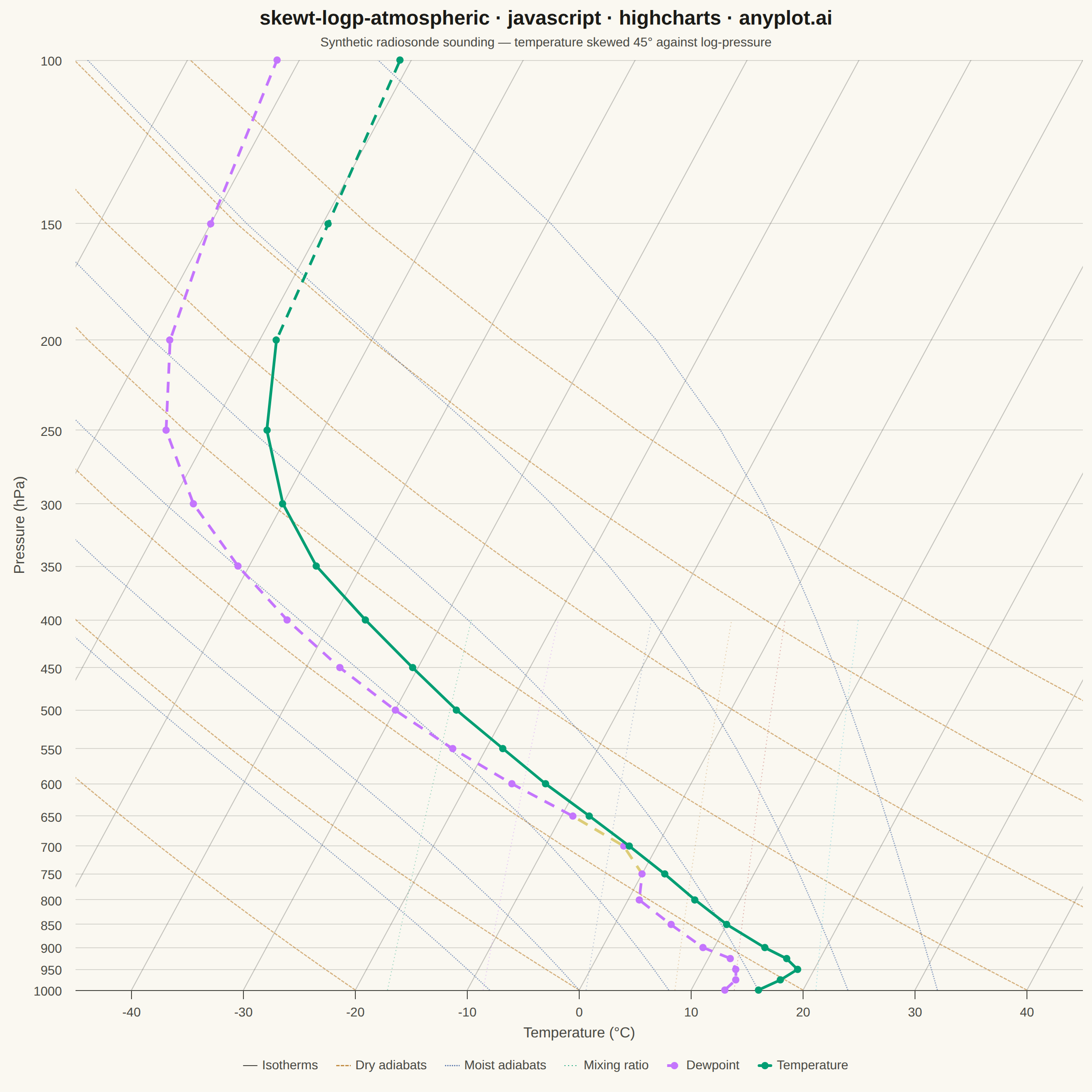
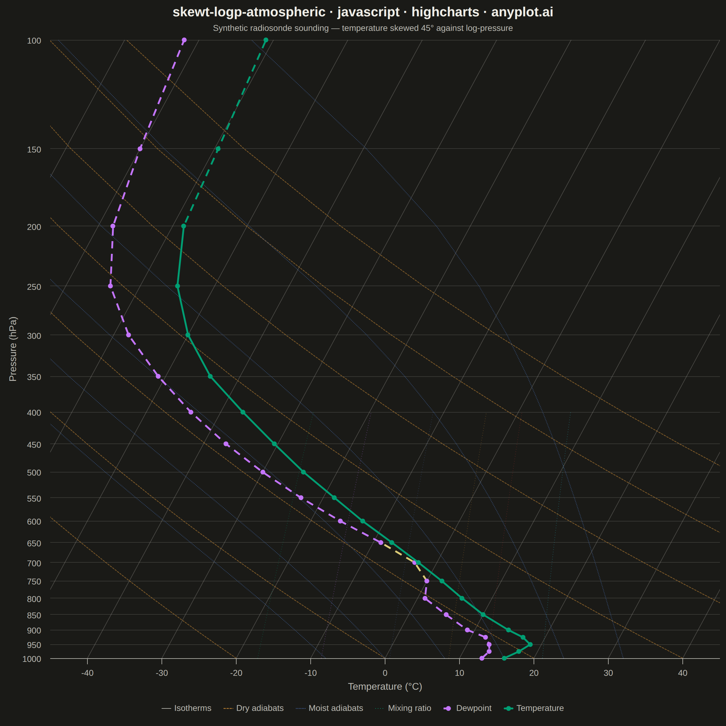
A Skew-T Log-P diagram is a specialized thermodynamic chart used in meteorology to display vertical atmospheric profiles. It features a logarithmic pressure axis (inverted, with surface at bottom) and temperature isotherms skewed 45 degrees to the right, allowing simultaneous visualization of temperature, dewpoint, and derived stability parameters. This diagram is essential for analyzing atmospheric soundings and assessing weather conditions.
// anyplot.ai
// skewt-logp-atmospheric: Skew-T Log-P Atmospheric Diagram
// Library: highcharts 12.6.0 | JavaScript 22.23.2
// Quality: 91/100 | Created: 2026-08-26

//# anyplot-orientation: square
const t = window.ANYPLOT_TOKENS;

// --- Thermodynamic helpers ---------------------------------------------------
const GAS_CONSTANT_DRY = 287.05; // J / (kg K)
const SPECIFIC_HEAT_DRY = 1005.7; // J / (kg K)
const LATENT_HEAT_VAPORIZATION = 2501000; // J / kg
const MIXING_RATIO_EPSILON = 0.622;
const SKEW = 45; // deg C shift per log10 decade of pressure — sets the isotherm slant

function skewX(tempC, pressureHpa) {
  return tempC + SKEW * Math.log10(1000 / pressureHpa);
}

function saturationVaporPressure(tempC) {
  return 6.112 * Math.exp((17.67 * tempC) / (tempC + 243.5));
}

function saturationMixingRatio(tempC, pressureHpa) {
  const vaporPressure = saturationVaporPressure(tempC);
  return (MIXING_RATIO_EPSILON * vaporPressure) / (pressureHpa - vaporPressure);
}

function mixingRatioToTemp(mixingRatio, pressureHpa) {
  const vaporPressure = (mixingRatio * pressureHpa) / (MIXING_RATIO_EPSILON + mixingRatio);
  const logTerm = Math.log(vaporPressure / 6.112);
  return (243.5 * logTerm) / (17.67 - logTerm);
}

function dryAdiabatTemp(potentialTempC, pressureHpa) {
  const potentialTempK = potentialTempC + 273.15;
  return potentialTempK * Math.pow(pressureHpa / 1000, GAS_CONSTANT_DRY / SPECIFIC_HEAT_DRY) - 273.15;
}

function moistLapseRate(tempK, pressureHpa) {
  const rs = saturationMixingRatio(tempK - 273.15, pressureHpa);
  const numerator = GAS_CONSTANT_DRY * tempK + LATENT_HEAT_VAPORIZATION * rs;
  const denominator = SPECIFIC_HEAT_DRY
    + (LATENT_HEAT_VAPORIZATION * LATENT_HEAT_VAPORIZATION * rs * MIXING_RATIO_EPSILON) / (GAS_CONSTANT_DRY * tempK * tempK);
  return numerator / (pressureHpa * denominator);
}

// Numerically integrates the saturated-adiabatic lapse rate from 1000 hPa
// through each sample pressure — moist adiabats have no closed-form solution.
function moistAdiabatCurve(startTempC, pressures) {
  let tempK = startTempC + 273.15;
  let pressure = 1000;
  return pressures.map((targetPressure) => {
    const steps = Math.max(1, Math.round(Math.abs(pressure - targetPressure) / 5));
    const step = (targetPressure - pressure) / steps;
    for (let i = 0; i < steps; i += 1) {
      tempK += moistLapseRate(tempK, pressure) * step;
      pressure += step;
    }
    return [skewX(tempK - 273.15, targetPressure), targetPressure];
  });
}

// --- Sounding data (synthetic radiosonde profile) ---------------------------
const pressureLevels = [1000, 975, 950, 925, 900, 850, 800, 750, 700, 650,
  600, 550, 500, 450, 400, 350, 300, 250, 200, 150, 100];
// Includes a shallow surface-based inversion (1000-950 hPa warms before
// cooling resumes) and a near-saturated layer around 700 hPa (dewpoint
// depression narrows to 0.5 degC) to showcase more of the diagram's range.
const temperatureC = [16, 17.5, 18.5, 17, 14.5, 10, 6, 2, -2.5, -7.5,
  -13, -18.5, -24.5, -30.5, -37, -44, -50, -55, -58.5, -59.5, -61];
const dewpointC = [13, 13.5, 13, 12, 9, 5, 1, 0, -3, -9,
  -16, -23, -30, -37, -44, -51, -58, -64, -68, -70, -72];

const temperaturePoints = pressureLevels.map((p, i) => [skewX(temperatureC[i], p), p]);
const dewpointPoints = pressureLevels.map((p, i) => [skewX(dewpointC[i], p), p]);

// --- Reference-line families (isotherms, adiabats, mixing ratios) -----------
const referencePressures = [];
for (let p = 1000; p >= 100; p -= 50) referencePressures.push(p);
const mixingRatioPressures = referencePressures.filter((p) => p >= 400);

const isothermSeries = [];
for (let tempC = -80; tempC <= 40; tempC += 10) {
  isothermSeries.push({
    name: "Isotherms",
    type: "line",
    data: [[skewX(tempC, 1000), 1000], [skewX(tempC, 100), 100]],
    color: t.inkSoft,
    opacity: 0.3,
    lineWidth: 1,
    showInLegend: tempC === -80,
    marker: { enabled: false },
    enableMouseTracking: false,
  });
}

const dryAdiabatSeries = [];
for (let potentialTempC = -20; potentialTempC <= 100; potentialTempC += 20) {
  dryAdiabatSeries.push({
    name: "Dry adiabats",
    type: "line",
    data: referencePressures.map((p) => [skewX(dryAdiabatTemp(potentialTempC, p), p), p]),
    color: t.palette[3],
    dashStyle: "ShortDash",
    lineWidth: 1.25,
    opacity: 0.6,
    showInLegend: potentialTempC === -20,
    marker: { enabled: false },
    enableMouseTracking: false,
  });
}

const moistAdiabatSeries = [];
for (let startTempC = -8; startTempC <= 32; startTempC += 8) {
  moistAdiabatSeries.push({
    name: "Moist adiabats",
    type: "line",
    data: moistAdiabatCurve(startTempC, referencePressures),
    color: t.palette[2],
    dashStyle: "ShortDot",
    lineWidth: 1.25,
    opacity: 0.6,
    showInLegend: startTempC === -8,
    marker: { enabled: false },
    enableMouseTracking: false,
  });
}

const mixingRatioSeries = [];
for (const mixingRatioGkg of [1, 2, 4, 7, 10, 16]) {
  mixingRatioSeries.push({
    name: "Mixing ratio",
    type: "line",
    data: mixingRatioPressures.map((p) => [skewX(mixingRatioToTemp(mixingRatioGkg / 1000, p), p), p]),
    color: t.muted,
    dashStyle: "Dot",
    lineWidth: 1,
    opacity: 0.4,
    showInLegend: mixingRatioGkg === 1,
    marker: { enabled: false },
    enableMouseTracking: false,
  });
}

// --- Chart -------------------------------------------------------------------
Highcharts.chart("container", {
  chart: { type: "line", backgroundColor: "transparent", animation: false,
           style: { fontFamily: "inherit" } },
  credits: { enabled: false },
  colors: t.palette,
  title: { text: "skewt-logp-atmospheric · javascript · highcharts · anyplot.ai",
           style: { color: t.ink, fontSize: "22px", fontWeight: "600" } },
  subtitle: { text: "Synthetic radiosonde sounding — temperature skewed 45° against log-pressure",
              style: { color: t.inkSoft, fontSize: "14px" } },
  xAxis: {
    min: -45,
    max: 45,
    gridLineWidth: 0,
    lineColor: t.inkSoft,
    tickColor: t.inkSoft,
    title: { text: "Temperature (°C)",
             style: { color: t.inkSoft, fontSize: "16px" } },
    labels: { style: { color: t.inkSoft, fontSize: "14px" } },
  },
  yAxis: {
    type: "logarithmic",
    reversed: true,
    min: 100,
    max: 1000,
    gridLineColor: t.grid,
    lineColor: t.inkSoft,
    tickColor: t.inkSoft,
    title: { text: "Pressure (hPa)", style: { color: t.inkSoft, fontSize: "16px" } },
    labels: { formatter() { return this.value; }, style: { color: t.inkSoft, fontSize: "14px" } },
  },
  legend: {
    itemStyle: { color: t.inkSoft, fontSize: "14px" },
    itemHoverStyle: { color: t.ink },
  },
  tooltip: {
    formatter() {
      return `${this.series.name}<br>Pressure: ${this.y} hPa`;
    },
  },
  plotOptions: { series: { animation: false } },
  series: [
    ...isothermSeries,
    ...dryAdiabatSeries,
    ...moistAdiabatSeries,
    ...mixingRatioSeries,
    {
      name: "Dewpoint",
      type: "line",
      data: dewpointPoints,
      color: t.palette[1],
      dashStyle: "Dash",
      lineWidth: 3,
      // Zones color-segment the 650-750 hPa band amber: dewpoint depression
      // narrows to ~0.5 degC there, i.e. a near-saturated (likely cloudy) layer.
      zoneAxis: "y",
      zones: [
        { value: 650, color: t.palette[1], dashStyle: "Dash" },
        { value: 750, color: t.amber, dashStyle: "Dash", lineWidth: 5 },
      ],
      marker: { enabled: true, symbol: "circle", radius: 4, fillColor: t.palette[1] },
    },
    {
      name: "Temperature",
      type: "line",
      data: temperaturePoints,
      color: t.palette[0],
      lineWidth: 3,
      // Zones dash the tropopause-and-above segment (<=200 hPa), where the
      // lapse rate flattens toward isothermal — a genuine per-segment
      // Highcharts feature rather than a second flat-colored line series.
      zoneAxis: "y",
      zones: [{ value: 200, color: t.palette[0], dashStyle: "Dash" }],
      marker: { enabled: true, symbol: "circle", radius: 4, fillColor: t.palette[0] },
    },
  ],
});
Runnable source as JSON, for any HTTP client: https://api.anyplot.ai/specs/skewt-logp-atmospheric/highcharts/code. Any spec id and library id listed in llms-full.txt fit the same URL shape; every URL below is complete and callable.
{
  "spec_id": "skewt-logp-atmospheric",
  "language": "javascript",
  "library": "highcharts",
  "page": "https://anyplot.ai/skewt-logp-atmospheric/javascript/highcharts",
  "hub": "https://anyplot.ai/skewt-logp-atmospheric",
  "code_json": "https://api.anyplot.ai/specs/skewt-logp-atmospheric/highcharts/code",
  "spec_json": "https://api.anyplot.ai/specs/skewt-logp-atmospheric",
  "render_light_png": "https://storage.googleapis.com/anyplot-images/plots/skewt-logp-atmospheric/javascript/highcharts/plot-light.png",
  "render_dark_png": "https://storage.googleapis.com/anyplot-images/plots/skewt-logp-atmospheric/javascript/highcharts/plot-dark.png",
  "interactive_light_html": "https://storage.googleapis.com/anyplot-images/plots/skewt-logp-atmospheric/javascript/highcharts/plot-light.html",
  "interactive_dark_html": "https://storage.googleapis.com/anyplot-images/plots/skewt-logp-atmospheric/javascript/highcharts/plot-dark.html",
  "quality_score": 91.0,
  "license": "MIT",
  "guide": "https://anyplot.ai/llms.txt"
}
Part of Skew-T Log-P Atmospheric Diagram on anyplot.ai.