The same plot in 14 other libraries — Python: Altair, Bokeh, lets-plot, Matplotlib, Plotly, plotnine, Pygal, Seaborn; Julia: Makie.jl; JavaScript: Chart.js, D3.js, Apache ECharts, Highcharts, MUI X Charts. Compare all 15 side by side: Skew-T Log-P Atmospheric Diagram in Python, R, Julia and JavaScript.
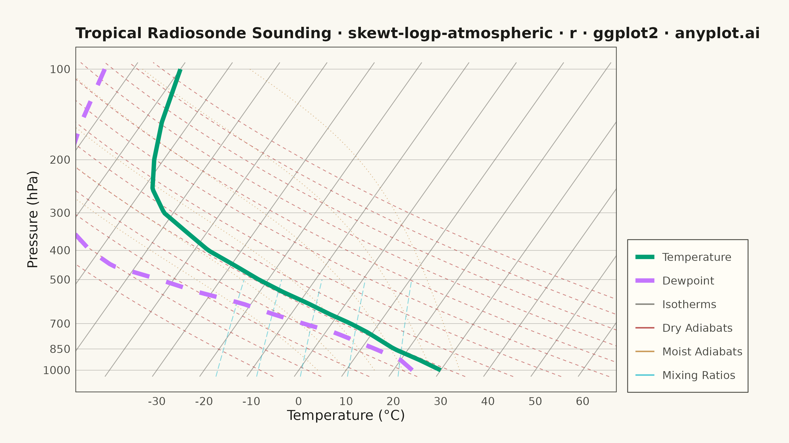
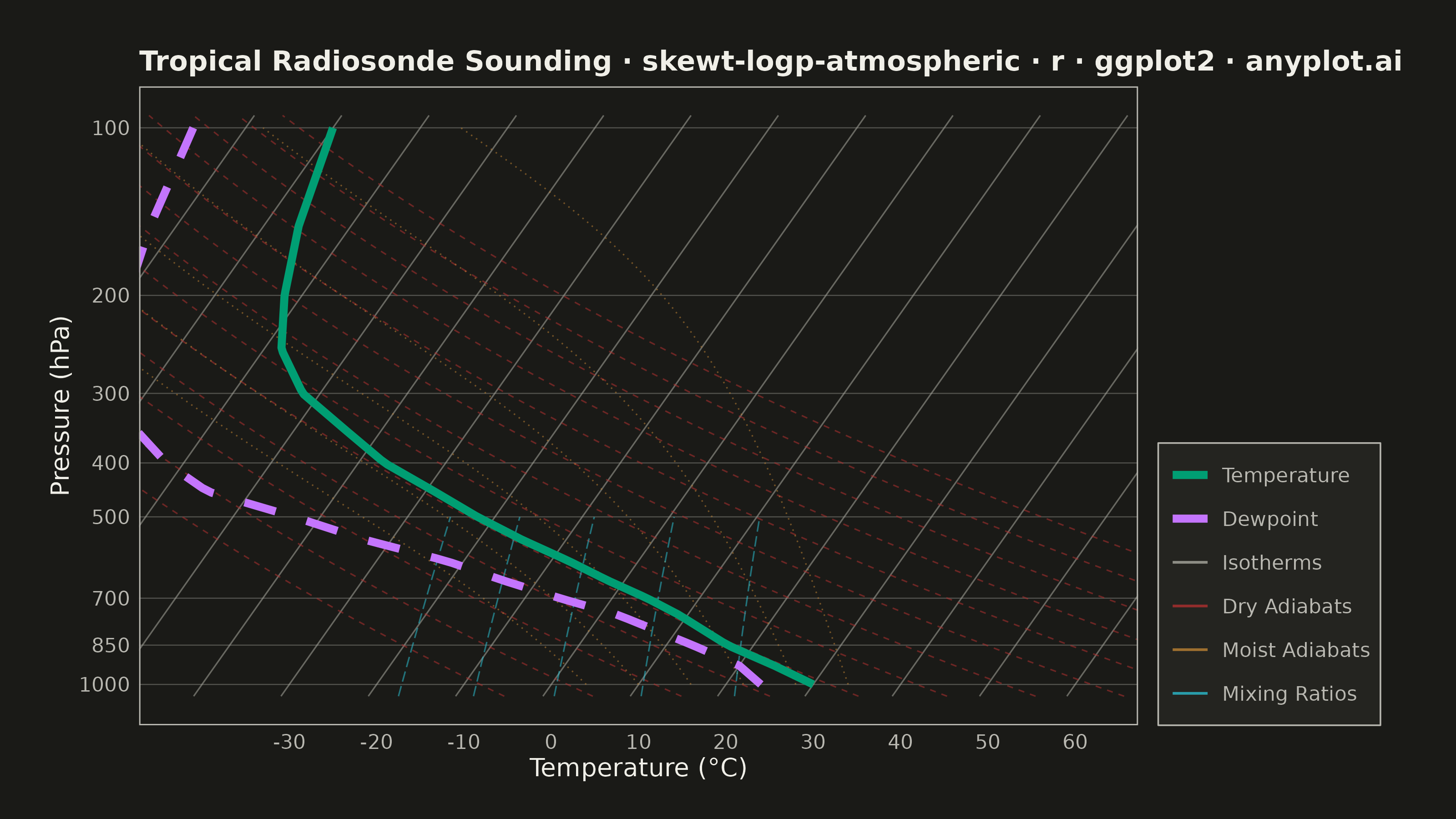
A Skew-T Log-P diagram is a specialized thermodynamic chart used in meteorology to display vertical atmospheric profiles. It features a logarithmic pressure axis (inverted, with surface at bottom) and temperature isotherms skewed 45 degrees to the right, allowing simultaneous visualization of temperature, dewpoint, and derived stability parameters. This diagram is essential for analyzing atmospheric soundings and assessing weather conditions.
#' anyplot.ai
#' skewt-logp-atmospheric: Skew-T Log-P Atmospheric Diagram
#' Library: ggplot2 3.5.1 | R 4.4.1
#' Quality: 90/100 | Created: 2026-05-21

library(ggplot2)
library(ragg)

set.seed(42)

# --- Theme tokens ------------------------------------------------------------
THEME       <- Sys.getenv("ANYPLOT_THEME", "light")
PAGE_BG     <- if (THEME == "light") "#FAF8F1" else "#1A1A17"
ELEVATED_BG <- if (THEME == "light") "#FFFDF6" else "#242420"
INK         <- if (THEME == "light") "#1A1A17" else "#F0EFE8"
INK_SOFT    <- if (THEME == "light") "#4A4A44" else "#B8B7B0"
INK_MUTED   <- if (THEME == "light") "#6B6A63" else "#A8A79F"
IMPRINT   <- c("#009E73", "#C475FD", "#4467A3", "#BD8233",
                 "#AE3030", "#2ABCCD", "#954477")

# --- Coordinate Helpers ------------------------------------------------------
# Y-axis: negative log10 of pressure so that high pressure (surface) sits at
# the bottom and low pressure (upper atm) sits at the top.
lp <- function(P_hpa) -log10(P_hpa)

# X-axis: temperature + skew offset to tilt isotherms 45°
SKEW <- 45   # °C per log10(P) decade
skewx <- function(T_c, P_hpa) T_c + SKEW * log10(1000 / P_hpa)

# --- Atmospheric Physics (Bolton 1980 approximations) -----------------------
es_hpa <- function(T_c) 6.112 * exp(17.67 * T_c / (T_c + 243.5))

ws_kgkg <- function(T_c, P_hpa) {
  es <- pmin(es_hpa(T_c), P_hpa * 0.99)
  0.622 * es / (P_hpa - es)
}

# Pseudo-adiabatic lapse rate (Euler integration, P decreasing = rising air)
moist_adiabat <- function(T0_c, P0 = 1000, Pend = 100, n = 200) {
  Lv <- 2.501e6; Rd <- 287.0; Cp <- 1004.0
  P_lev <- exp(seq(log(P0), log(Pend), length.out = n))
  T_c <- numeric(n)
  T_c[1] <- T0_c
  for (i in 2:n) {
    T_K  <- T_c[i - 1] + 273.15
    P    <- P_lev[i - 1]
    ws   <- ws_kgkg(T_c[i - 1], P)
    num  <- Rd * T_K / P + Lv * ws / P
    den  <- Cp + Lv^2 * ws * 0.622 / (Rd * T_K^2)
    T_c[i] <- T_c[i - 1] + (num / den) * (P_lev[i] - P)
  }
  data.frame(P = P_lev, T_c = T_c)
}

# --- Radiosonde Sounding (tropical pre-storm profile) -----------------------
pres_obs <- c(1000, 925, 850, 750, 700, 650, 600, 550, 500, 450,
              400, 350, 300, 250, 200, 150, 100)
temp_obs <- c(30, 24, 17, 9, 4, -2, -8, -15, -22, -29,
              -37, -44, -52, -58, -62, -66, -70)
dew_obs  <- c(24, 20, 13, 2, -6, -14, -22, -33, -43, -55,
              -62, -68, -73, -77, -80, -83, -86)

# Smooth interpolation in log-P space
p_fine  <- exp(seq(log(max(pres_obs)), log(min(pres_obs)), length.out = 120))
T_fine  <- approx(log(pres_obs), temp_obs, xout = log(p_fine))$y
Td_fine <- approx(log(pres_obs), dew_obs,  xout = log(p_fine))$y

sounding <- data.frame(
  y   = lp(p_fine),
  xT  = skewx(T_fine,  p_fine),
  xTd = skewx(Td_fine, p_fine)
)

# --- Reference Lines --------------------------------------------------------
p_ref <- exp(seq(log(1050), log(95), length.out = 400))
y_ref <- lp(p_ref)

# Temperature isotherms — mapped to series for legend
iso_df <- do.call(rbind, lapply(seq(-80, 60, by = 10), function(T0) {
  data.frame(group = T0, y = y_ref, x = skewx(T0, p_ref), series = "Isotherms")
}))

# Dry adiabats (Poisson: T_K = theta * (P/1000)^0.286)
dry_df <- do.call(rbind, lapply(seq(265, 390, by = 10), function(th_K) {
  T_c <- th_K * (p_ref / 1000)^0.286 - 273.15
  data.frame(group = th_K, y = y_ref, x = skewx(T_c, p_ref), series = "Dry Adiabats")
}))

# Moist pseudo-adiabats starting from the surface
moist_df <- do.call(rbind, lapply(c(4, 10, 16, 22, 28, 34), function(T0) {
  df       <- moist_adiabat(T0, P0 = 1000, Pend = 100, n = 200)
  df$group <- T0
  df$y     <- lp(df$P)
  df$x     <- skewx(df$T_c, df$P)
  df$series <- "Moist Adiabats"
  df
}))

# Saturation mixing ratio lines (lower troposphere only)
p_mix  <- exp(seq(log(1050), log(500), length.out = 200))
mix_df <- do.call(rbind, lapply(c(1, 2, 4, 8, 16), function(w_gpkg) {
  w_kg <- w_gpkg / 1000
  es   <- w_kg * p_mix / (0.622 + w_kg)
  T_c  <- 243.5 * log(es / 6.112) / (17.67 - log(es / 6.112))
  data.frame(group = w_gpkg, y = lp(p_mix), x = skewx(T_c, p_mix),
             series = "Mixing Ratios")
}))

# --- Y-axis Setup (log-pressure labels) -------------------------------------
p_labeled <- c(1000, 850, 700, 500, 400, 300, 200, 100)
y_breaks  <- lp(p_labeled)
y_labels  <- as.character(p_labeled)

# Isobar positions for horizontal reference lines
y_isobars <- lp(c(1000, 850, 700, 500, 400, 300, 200, 100))

# Plot y limits (from 1050 hPa at bottom to 95 hPa at top)
y_lo <- lp(1050)  # ≈ -3.021
y_hi <- lp(95)    # ≈ -1.978

# --- Long-form sounding for colour + linetype legend -----------------------
snd_long <- rbind(
  data.frame(y = sounding$y, x = sounding$xT,  series = "Temperature"),
  data.frame(y = sounding$y, x = sounding$xTd, series = "Dewpoint")
)

# --- Combined scale values (order controls legend display) ------------------
series_order <- c("Temperature", "Dewpoint", "Isotherms",
                  "Dry Adiabats", "Moist Adiabats", "Mixing Ratios")

color_values <- c(
  "Temperature"   = IMPRINT[1],   # #009E73 green
  "Dewpoint"      = IMPRINT[2],   # #C475FD orange-red
  "Isotherms"     = INK_MUTED,      # gray, theme-adaptive
  "Dry Adiabats"  = IMPRINT[5],   # #AE3030 amber
  "Moist Adiabats"= IMPRINT[4],   # #BD8233 purple (distinct from sky blue)
  "Mixing Ratios" = IMPRINT[6]    # #2ABCCD sky blue
)

linetype_values <- c(
  "Temperature"   = "solid",
  "Dewpoint"      = "dashed",
  "Isotherms"     = "solid",
  "Dry Adiabats"  = "dashed",
  "Moist Adiabats"= "dotted",
  "Mixing Ratios" = "longdash"
)

# --- Plot -------------------------------------------------------------------
p <- ggplot() +
  # Horizontal isobars at standard levels
  geom_hline(
    yintercept = y_isobars,
    color = INK_MUTED, linewidth = 0.2, alpha = 0.40
  ) +
  # Reference lines — mapped to series aesthetic for unified legend
  geom_path(
    data = iso_df,
    aes(x = x, y = y, group = group, color = series, linetype = series),
    linewidth = 0.28, alpha = 0.55
  ) +
  geom_path(
    data = dry_df,
    aes(x = x, y = y, group = group, color = series, linetype = series),
    linewidth = 0.28, alpha = 0.55
  ) +
  geom_path(
    data = moist_df,
    aes(x = x, y = y, group = group, color = series, linetype = series),
    linewidth = 0.28, alpha = 0.55
  ) +
  geom_path(
    data = mix_df,
    aes(x = x, y = y, group = group, color = series, linetype = series),
    linewidth = 0.28, alpha = 0.55
  ) +
  # Main sounding profiles with legend (Temperature = first/brand colour)
  geom_path(
    data = snd_long,
    aes(x = x, y = y, color = series, linetype = series),
    linewidth = 1.5
  ) +
  scale_color_manual(
    name   = NULL,
    values = color_values,
    breaks = series_order
  ) +
  scale_linetype_manual(
    name   = NULL,
    values = linetype_values,
    breaks = series_order
  ) +
  scale_y_continuous(
    breaks = y_breaks,
    labels = y_labels,
    limits = c(y_lo, y_hi)
  ) +
  scale_x_continuous(breaks = seq(-30, 60, by = 10)) +
  coord_cartesian(xlim = c(-42, 62)) +
  labs(
    x     = "Temperature (°C)",
    y     = "Pressure (hPa)",
    title = paste0(
      "Tropical Radiosonde Sounding · ",
      "skewt-logp-atmospheric · r · ggplot2 · anyplot.ai"
    )
  ) +
  theme_minimal(base_size = 8) +
  theme(
    plot.background   = element_rect(fill = PAGE_BG, color = PAGE_BG),
    panel.background  = element_rect(fill = PAGE_BG, color = NA),
    panel.grid.major  = element_blank(),
    panel.grid.minor  = element_blank(),
    panel.border      = element_rect(color = INK_SOFT, fill = NA, linewidth = 0.5),
    axis.title        = element_text(color = INK,      size = 10),
    axis.text         = element_text(color = INK_SOFT, size = 8),
    plot.title        = element_text(color = INK,      size = 11, face = "bold"),
    legend.background = element_rect(fill = ELEVATED_BG, color = INK_SOFT,
                                     linewidth = 0.3),
    legend.text       = element_text(color = INK_SOFT, size = 8),
    legend.position.inside = c(0.88, 0.05),
    legend.justification   = c(1, 0),
    plot.margin       = margin(20, 30, 15, 20)
  ) +
  guides(
    color = guide_legend(
      override.aes = list(
        linewidth = c(1.5, 1.5, 0.5, 0.5, 0.5, 0.5),
        alpha     = c(1.0, 1.0, 0.8, 0.8, 0.8, 0.8)
      )
    ),
    linetype = "none"
  )

# --- Save -------------------------------------------------------------------
ggsave(
  filename = sprintf("plot-%s.png", THEME),
  plot     = p,
  device   = ragg::agg_png,
  width    = 8,
  height   = 4.5,
  units    = "in",
  dpi      = 400
)
Runnable source as JSON, for any HTTP client: https://api.anyplot.ai/specs/skewt-logp-atmospheric/ggplot2/code. Any spec id and library id listed in llms-full.txt fit the same URL shape; every URL below is complete and callable.
{
  "spec_id": "skewt-logp-atmospheric",
  "language": "r",
  "library": "ggplot2",
  "page": "https://anyplot.ai/skewt-logp-atmospheric/r/ggplot2",
  "hub": "https://anyplot.ai/skewt-logp-atmospheric",
  "code_json": "https://api.anyplot.ai/specs/skewt-logp-atmospheric/ggplot2/code",
  "spec_json": "https://api.anyplot.ai/specs/skewt-logp-atmospheric",
  "render_light_png": "https://storage.googleapis.com/anyplot-images/plots/skewt-logp-atmospheric/r/ggplot2/plot-light.png",
  "render_dark_png": "https://storage.googleapis.com/anyplot-images/plots/skewt-logp-atmospheric/r/ggplot2/plot-dark.png",
  "quality_score": 90.0,
  "license": "MIT",
  "guide": "https://anyplot.ai/llms.txt"
}
Part of Skew-T Log-P Atmospheric Diagram on anyplot.ai.