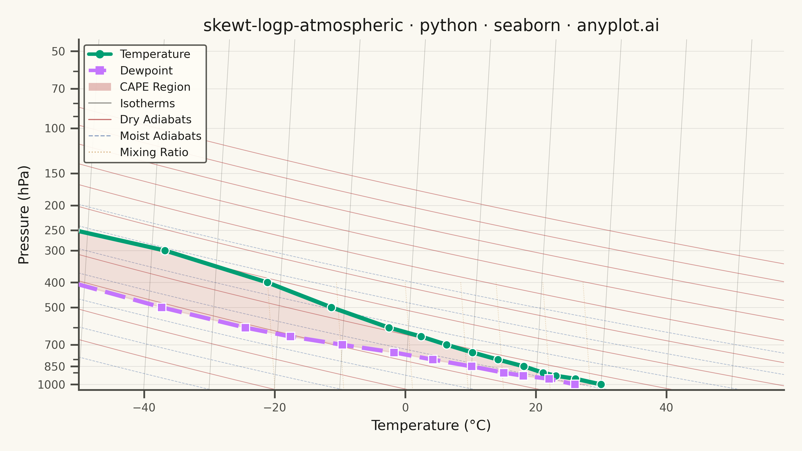
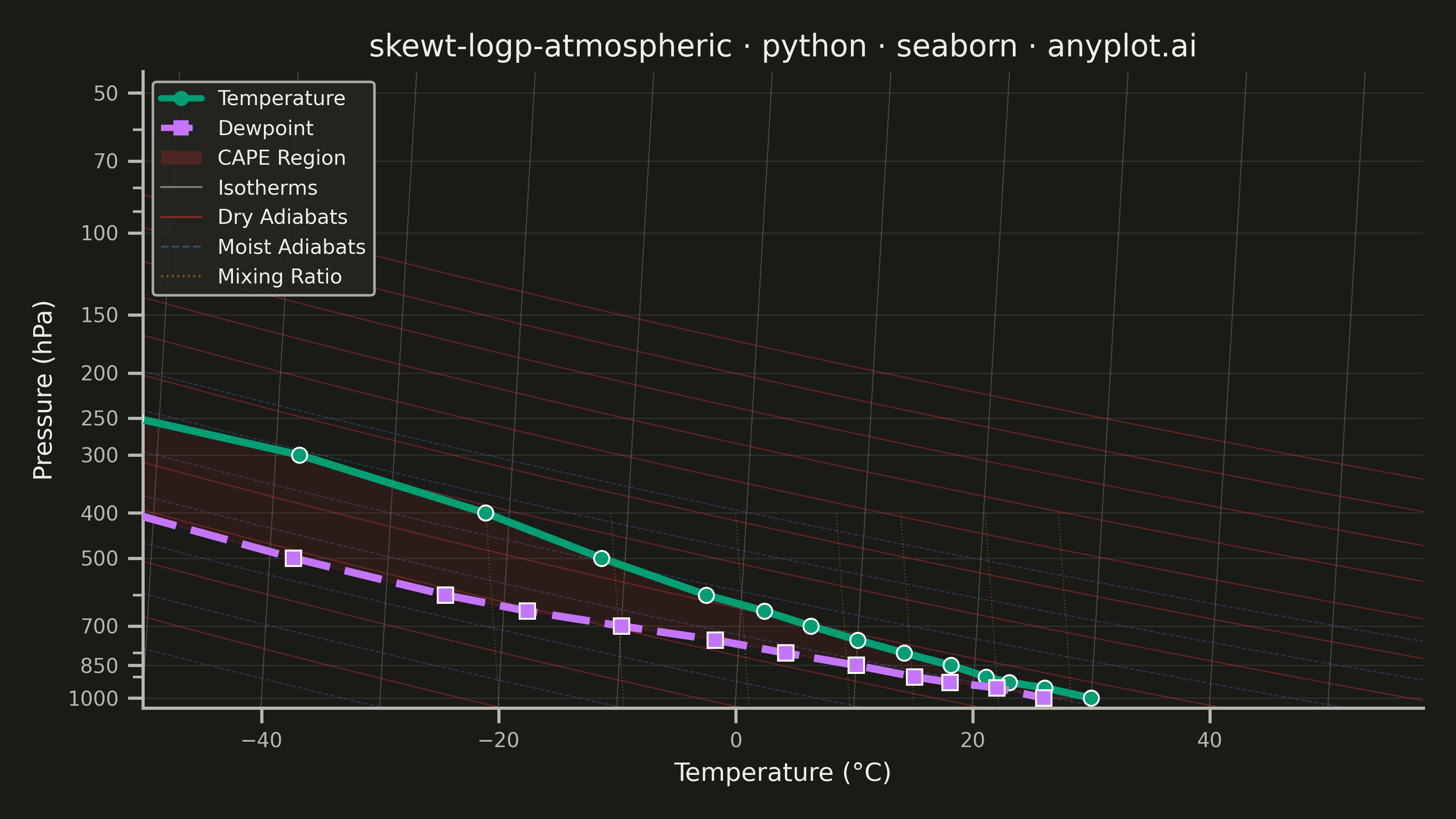
A Skew-T Log-P diagram is a specialized thermodynamic chart used in meteorology to display vertical atmospheric profiles. It features a logarithmic pressure axis (inverted, with surface at bottom) and temperature isotherms skewed 45 degrees to the right, allowing simultaneous visualization of temperature, dewpoint, and derived stability parameters. This diagram is essential for analyzing atmospheric soundings and assessing weather conditions.
""" anyplot.ai
skewt-logp-atmospheric: Skew-T Log-P Atmospheric Diagram
Library: seaborn 0.13.2 | Python 3.13.13
Quality: 85/100 | Updated: 2026-05-21
"""

import os

import matplotlib.pyplot as plt
import numpy as np
import pandas as pd
import seaborn as sns
from matplotlib.lines import Line2D
from matplotlib.patches import Patch
from matplotlib.ticker import ScalarFormatter


# Theme tokens
THEME = os.getenv("ANYPLOT_THEME", "light")
PAGE_BG = "#FAF8F1" if THEME == "light" else "#1A1A17"
ELEVATED_BG = "#FFFDF6" if THEME == "light" else "#242420"
INK = "#1A1A17" if THEME == "light" else "#F0EFE8"
INK_SOFT = "#4A4A44" if THEME == "light" else "#B8B7B0"

IMPRINT = ["#009E73", "#C475FD", "#4467A3", "#BD8233", "#AE3030", "#2ABCCD", "#954477"]

sns.set_theme(
    style="ticks",
    rc={
        "figure.facecolor": PAGE_BG,
        "axes.facecolor": PAGE_BG,
        "axes.edgecolor": INK_SOFT,
        "axes.labelcolor": INK,
        "text.color": INK,
        "xtick.color": INK_SOFT,
        "ytick.color": INK_SOFT,
        "grid.color": INK,
        "grid.alpha": 0.10,
        "legend.facecolor": ELEVATED_BG,
        "legend.edgecolor": INK_SOFT,
    },
)

# Data: tropical atmospheric sounding — 19 levels from surface (1000 hPa) to stratosphere (50 hPa)
np.random.seed(42)
pressure = np.array([1000, 950, 925, 900, 850, 800, 750, 700, 650, 600, 500, 400, 300, 250, 200, 150, 100, 70, 50])
temperature = np.array([30, 26, 23, 21, 18, 14, 10, 6, 2, -3, -12, -22, -38, -52, -60, -65, -75, -65, -55])
dewpoint = np.array([26, 22, 18, 15, 10, 4, -2, -10, -18, -25, -38, -52, -60, -70, -75, -80, -85, -90, -90])

# Figure with logarithmic inverted pressure axis
fig, ax = plt.subplots(figsize=(8, 4.5), dpi=400)

ax.set_yscale("log")
ax.set_ylim(1050, 45)
ax.set_xlim(-50, 58)

# Skew-T transform: x_plot = T + tan(45°) * ln(p0/p)
skew_slope = np.tan(np.radians(45))
p_bg = np.logspace(np.log10(45), np.log10(1050), 150)

# Isotherms — seaborn lineplot with units for multi-line rendering (seaborn-idiomatic)
iso_frames = []
for t in np.arange(-80, 65, 10):
    x_iso = t + skew_slope * np.log(1000 / p_bg)
    iso_frames.append(pd.DataFrame({"x": x_iso, "pressure": p_bg, "T": t}))
df_iso = pd.concat(iso_frames, ignore_index=True)
sns.lineplot(
    data=df_iso,
    x="x",
    y="pressure",
    units="T",
    estimator=None,
    color=INK_SOFT,
    linewidth=0.4,
    alpha=0.30,
    ax=ax,
    zorder=1,
    legend=False,
)

# Dry adiabats (potential temperature θ = const) — seaborn lineplot
dry_frames = []
for theta in np.arange(250, 470, 20):
    t_dry = theta * (p_bg / 1000) ** 0.286 - 273.15
    x_dry = t_dry + skew_slope * np.log(1000 / p_bg)
    dry_frames.append(pd.DataFrame({"x": x_dry, "pressure": p_bg, "theta": theta}))
df_dry = pd.concat(dry_frames, ignore_index=True)
sns.lineplot(
    data=df_dry,
    x="x",
    y="pressure",
    units="theta",
    estimator=None,
    color=IMPRINT[4],
    linewidth=0.5,
    alpha=0.50,
    ax=ax,
    zorder=1,
    legend=False,
)

# Moist adiabats (equivalent potential temperature θ_e = const) — seaborn lineplot
moist_frames = []
for theta_e in np.arange(270, 400, 20):
    t_moist = (theta_e - 30) * (p_bg / 1000) ** 0.30 - 273.15
    x_moist = t_moist + skew_slope * np.log(1000 / p_bg)
    moist_frames.append(pd.DataFrame({"x": x_moist, "pressure": p_bg, "theta_e": theta_e}))
df_moist = pd.concat(moist_frames, ignore_index=True)
sns.lineplot(
    data=df_moist,
    x="x",
    y="pressure",
    units="theta_e",
    estimator=None,
    color=IMPRINT[2],
    linewidth=0.5,
    alpha=0.40,
    linestyle="--",
    ax=ax,
    zorder=1,
    legend=False,
)

# Mixing ratio lines (w = const, g/kg) — lower troposphere only — seaborn lineplot
p_mix = np.logspace(np.log10(400), np.log10(1050), 60)
mix_frames = []
for w in [1, 2, 4, 7, 10, 16, 24]:
    t_mix = 35 * np.log10(w) - 20 + 5 * np.log10(p_mix / 1000)
    x_mix = t_mix + skew_slope * np.log(1000 / p_mix)
    mix_frames.append(pd.DataFrame({"x": x_mix, "pressure": p_mix, "w": w}))
df_mix = pd.concat(mix_frames, ignore_index=True)
sns.lineplot(
    data=df_mix,
    x="x",
    y="pressure",
    units="w",
    estimator=None,
    color=IMPRINT[3],
    linewidth=0.5,
    alpha=0.40,
    linestyle=":",
    ax=ax,
    zorder=1,
    legend=False,
)

# Apply skew transform to sounding data
x_temp = temperature + skew_slope * np.log(1000 / pressure)
x_dew = dewpoint + skew_slope * np.log(1000 / pressure)

# CAPE region: shade area between temperature and dewpoint profiles (T > Td = instability)
ax.fill_betweenx(pressure, x_dew, x_temp, alpha=0.12, color=IMPRINT[4], zorder=2)

df = pd.DataFrame(
    {
        "x": np.concatenate([x_temp, x_dew]),
        "pressure": np.concatenate([pressure, pressure]),
        "profile": ["Temperature"] * len(pressure) + ["Dewpoint"] * len(pressure),
    }
)

# Plot sounding profiles with seaborn lineplot (hue + style + markers = seaborn-idiomatic)
sns.lineplot(
    data=df,
    x="x",
    y="pressure",
    hue="profile",
    style="profile",
    markers={"Temperature": "o", "Dewpoint": "s"},
    dashes={"Temperature": "", "Dewpoint": (5, 2)},
    palette={"Temperature": IMPRINT[0], "Dewpoint": IMPRINT[1]},
    linewidth=3,
    markersize=6,
    ax=ax,
    zorder=5,
    legend=False,
)

# Pressure axis ticks and formatting
ax.yaxis.set_major_formatter(ScalarFormatter())
display_ticks = [1000, 850, 700, 500, 400, 300, 250, 200, 150, 100, 70, 50]
ax.set_yticks(display_ticks)
ax.set_yticklabels([str(p) for p in display_ticks])

# Labels and title
ax.set_xlabel("Temperature (°C)", fontsize=10, color=INK)
ax.set_ylabel("Pressure (hPa)", fontsize=10, color=INK)
ax.set_title("skewt-logp-atmospheric · python · seaborn · anyplot.ai", fontsize=12, fontweight="medium", color=INK)
ax.tick_params(axis="both", labelsize=8, colors=INK_SOFT)

sns.despine(ax=ax, top=True, right=True)
ax.spines["left"].set_color(INK_SOFT)
ax.spines["bottom"].set_color(INK_SOFT)
ax.yaxis.grid(True, alpha=0.10, linewidth=0.5, color=INK)

# Legend — upper-left where 100-200 hPa data is sparse (reduces crowding with mixing ratio lines)
legend_handles = [
    Line2D([0], [0], color=IMPRINT[0], lw=2.5, marker="o", markersize=5, label="Temperature"),
    Line2D([0], [0], color=IMPRINT[1], lw=2.5, linestyle=(0, (5, 2)), marker="s", markersize=5, label="Dewpoint"),
    Patch(facecolor=IMPRINT[4], alpha=0.30, edgecolor="none", label="CAPE Region"),
    Line2D([0], [0], color=INK_SOFT, lw=0.8, alpha=0.6, label="Isotherms"),
    Line2D([0], [0], color=IMPRINT[4], lw=0.8, alpha=0.7, label="Dry Adiabats"),
    Line2D([0], [0], color=IMPRINT[2], lw=0.8, alpha=0.6, linestyle="--", label="Moist Adiabats"),
    Line2D([0], [0], color=IMPRINT[3], lw=0.8, alpha=0.6, linestyle=":", label="Mixing Ratio"),
]
ax.legend(
    handles=legend_handles, loc="upper left", fontsize=8, framealpha=0.92, facecolor=ELEVATED_BG, edgecolor=INK_SOFT
)

plt.tight_layout()
plt.savefig(f"plot-{THEME}.png", dpi=400, facecolor=PAGE_BG)
Runnable source as JSON, for any HTTP client: https://api.anyplot.ai/specs/skewt-logp-atmospheric/seaborn/code. Any spec id and library id listed in llms-full.txt fit the same URL shape; every URL below is complete and callable.
{
  "spec_id": "skewt-logp-atmospheric",
  "language": "python",
  "library": "seaborn",
  "page": "https://anyplot.ai/skewt-logp-atmospheric/python/seaborn",
  "hub": "https://anyplot.ai/skewt-logp-atmospheric",
  "code_json": "https://api.anyplot.ai/specs/skewt-logp-atmospheric/seaborn/code",
  "spec_json": "https://api.anyplot.ai/specs/skewt-logp-atmospheric",
  "render_light_png": "https://storage.googleapis.com/anyplot-images/plots/skewt-logp-atmospheric/python/seaborn/plot-light.png",
  "render_dark_png": "https://storage.googleapis.com/anyplot-images/plots/skewt-logp-atmospheric/python/seaborn/plot-dark.png",
  "quality_score": 85.0,
  "license": "MIT",
  "guide": "https://anyplot.ai/llms.txt"
}
Part of Skew-T Log-P Atmospheric Diagram on anyplot.ai.