The same plot in 14 other libraries — JavaScript: Chart.js, Apache ECharts, Highcharts, MUI X Charts; Python: Altair, Bokeh, lets-plot, Matplotlib, Plotly, plotnine, Pygal, Seaborn; R: ggplot2; Julia: Makie.jl. Compare all 15 side by side: Skew-T Log-P Atmospheric Diagram in Python, R, Julia and JavaScript.
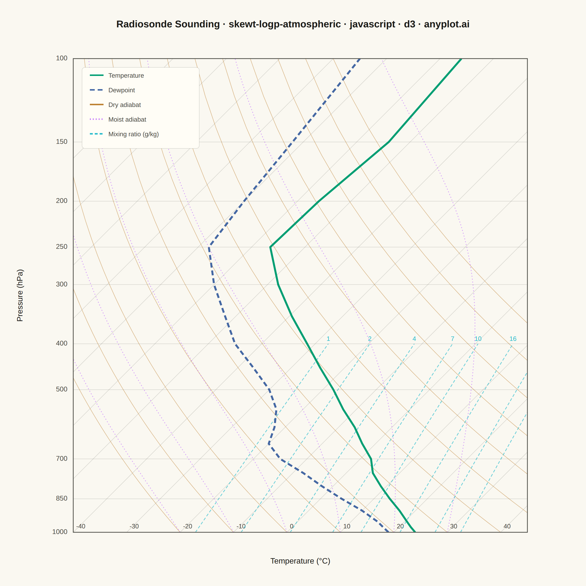
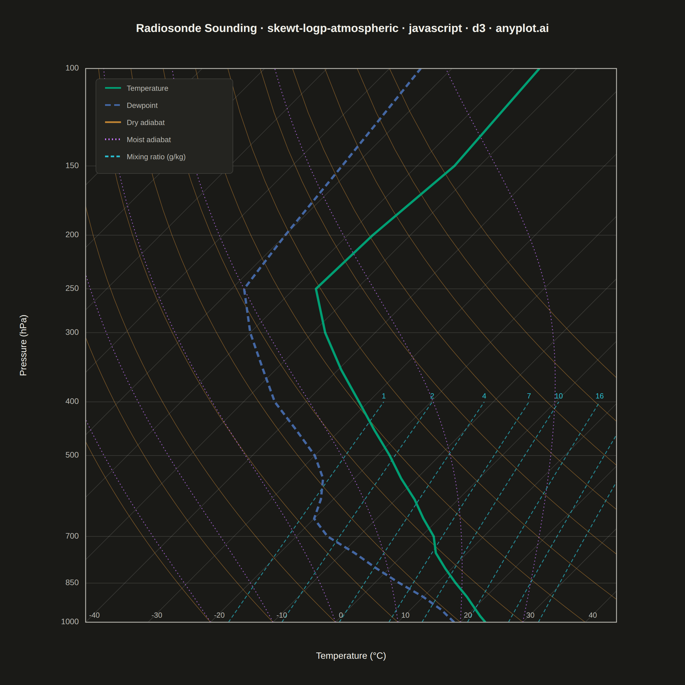
A Skew-T Log-P diagram is a specialized thermodynamic chart used in meteorology to display vertical atmospheric profiles. It features a logarithmic pressure axis (inverted, with surface at bottom) and temperature isotherms skewed 45 degrees to the right, allowing simultaneous visualization of temperature, dewpoint, and derived stability parameters. This diagram is essential for analyzing atmospheric soundings and assessing weather conditions.
// anyplot.ai
// skewt-logp-atmospheric: Skew-T Log-P Atmospheric Diagram
// Library: d3 7.9.0 | JavaScript 22.23.2
// Quality: 90/100 | Created: 2026-08-26

//# anyplot-orientation: square

const t = window.ANYPLOT_TOKENS;
const { width, height } = window.ANYPLOT_SIZE;
const margin = { top: 120, right: 120, bottom: 110, left: 150 };
const iw = width - margin.left - margin.right;
const ih = height - margin.top - margin.bottom;

// --- Data: radiosonde sounding (in-memory, deterministic) ------------------
// Classic "dry mid-level" convective sounding shape: dewpoint tracks the
// temperature closely near the surface, then diverges sharply around 700 hPa
// (a dry layer), and both cool through the troposphere toward the tropopause.
const sounding = [
  { p: 1000, temp: 24.0, dew: 19.0 },
  { p: 975, temp: 22.2, dew: 17.0 },
  { p: 950, temp: 20.5, dew: 15.0 },
  { p: 900, temp: 17.0, dew: 10.0 },
  { p: 850, temp: 13.0, dew: 4.0 },
  { p: 800, temp: 9.0, dew: -2.0 },
  { p: 750, temp: 5.0, dew: -8.0 },
  { p: 700, temp: 2.0, dew: -15.0 },
  { p: 650, temp: -2.5, dew: -20.0 },
  { p: 600, temp: -7.0, dew: -22.0 },
  { p: 550, temp: -12.5, dew: -25.0 },
  { p: 500, temp: -18.0, dew: -30.0 },
  { p: 450, temp: -24.5, dew: -37.0 },
  { p: 400, temp: -31.5, dew: -45.0 },
  { p: 350, temp: -39.5, dew: -52.0 },
  { p: 300, temp: -48.0, dew: -60.0 },
  { p: 250, temp: -56.5, dew: -68.0 },
  { p: 200, temp: -56.0, dew: -70.0 },
  { p: 150, temp: -54.0, dew: -72.0 },
  { p: 100, temp: -56.0, dew: -75.0 },
];

// --- Scales & skew transform -------------------------------------------------
// Pressure: logarithmic, inverted (1000 hPa surface at bottom, 100 hPa at top)
const yScale = d3.scaleLog().domain([1000, 100]).range([ih, 0]);
// Temperature: linear reference axis, evaluated at the surface (p = 1000 hPa)
const xScale = d3.scaleLinear().domain([-40, 45]).range([0, iw]);
const SKEW = 1; // 1 px right-shift per 1 px of height climbed -> 45-degree isotherms
function toX(tempC, p) {
  return xScale(tempC) + (ih - yScale(p)) * SKEW;
}
function toY(p) {
  return yScale(p);
}
const skewLine = d3.line().x((d) => toX(d[1], d[0])).y((d) => toY(d[0]));

// --- Thermodynamic reference curves -----------------------------------------
// Dry adiabat: constant potential temperature theta, T(p) = theta_K * (p/1000)^0.286
function dryAdiabatPoints(thetaC) {
  const thetaK = thetaC + 273.15;
  const pts = [];
  for (let p = 1000; p >= 100; p -= 20) pts.push([p, thetaK * Math.pow(p / 1000, 0.286) - 273.15]);
  return pts;
}

// Moist (pseudo-)adiabat: integrate the saturated-adiabatic lapse rate upward
// from a surface temperature, conserving equivalent potential temperature.
const RD = 287.05;
const CP = 1005.7;
const LV = 2.501e6;
const EPS = 0.622;
function saturationVaporPressure(tempC) {
  return 6.112 * Math.exp((17.67 * tempC) / (tempC + 243.5)); // Bolton (1980), hPa
}
function moistAdiabatPoints(startTempC) {
  const pts = [[1000, startTempC]];
  let tempK = startTempC + 273.15;
  let p = 1000;
  const dp = -4;
  while (p > 100) {
    const es = saturationVaporPressure(tempK - 273.15);
    const ws = (EPS * es) / (p - es);
    const numerator = RD * tempK + LV * ws;
    const denominator = CP + (LV * LV * ws * EPS) / (RD * tempK * tempK);
    tempK += (numerator / (denominator * p)) * dp;
    p += dp;
    pts.push([p, tempK - 273.15]);
  }
  return pts;
}

// Mixing ratio line: constant saturation mixing ratio w (g/kg) -> invert Bolton
function mixingRatioT(w, p) {
  const es = (w * p) / (622 + w);
  const logRatio = Math.log(es / 6.112);
  return (243.5 * logRatio) / (17.67 - logRatio);
}
function mixingRatioPoints(w) {
  const pts = [];
  for (let p = 1000; p >= 400; p -= 20) pts.push([p, mixingRatioT(w, p)]);
  return pts;
}

// --- SVG mount ---------------------------------------------------------------
const svg = d3.select("#container").append("svg").attr("width", width).attr("height", height);
const g = svg.append("g").attr("transform", `translate(${margin.left},${margin.top})`);

svg
  .append("clipPath")
  .attr("id", "plot-clip")
  .append("rect")
  .attr("x", 0)
  .attr("y", 0)
  .attr("width", iw)
  .attr("height", ih);
const clipped = g.append("g").attr("clip-path", "url(#plot-clip)");

// --- Isobars (horizontal pressure gridlines) ---------------------------------
const isobarLevels = [1000, 850, 700, 500, 400, 300, 250, 200, 150, 100];
g.append("g")
  .selectAll("line")
  .data(isobarLevels)
  .join("line")
  .attr("x1", 0)
  .attr("x2", iw)
  .attr("y1", (p) => toY(p))
  .attr("y2", (p) => toY(p))
  .attr("stroke", t.grid)
  .attr("stroke-width", 1);
g.append("g")
  .selectAll("text")
  .data(isobarLevels)
  .join("text")
  .attr("x", -12)
  .attr("y", (p) => toY(p))
  .attr("text-anchor", "end")
  .attr("dominant-baseline", "middle")
  .attr("fill", t.inkSoft)
  .style("font-size", "14px")
  .text((p) => `${p}`);

// --- Isotherms (straight, skewed 45 degrees) ---------------------------------
const isotherms = d3.range(-110, 51, 10);
clipped
  .selectAll("path.isotherm")
  .data(isotherms)
  .join("path")
  .attr("class", "isotherm")
  .attr("d", (tempC) => skewLine([[1000, tempC], [100, tempC]]))
  .attr("fill", "none")
  .attr("stroke", t.grid)
  .attr("stroke-width", 1);
clipped
  .selectAll("text.isotherm-label")
  .data(d3.range(-40, 41, 10))
  .join("text")
  .attr("class", "isotherm-label")
  .attr("x", (tempC) => toX(tempC, 1000) + 6)
  .attr("y", ih - 8)
  .attr("fill", t.inkSoft)
  .style("font-size", "13px")
  .text((tempC) => `${tempC}`);

// --- Dry adiabats --------------------------------------------------------------
const dryAdiabatThetas = d3.range(-20, 101, 10);
clipped
  .selectAll("path.dry-adiabat")
  .data(dryAdiabatThetas)
  .join("path")
  .attr("class", "dry-adiabat")
  .attr("d", (theta) => skewLine(dryAdiabatPoints(theta)))
  .attr("fill", "none")
  .attr("stroke", t.palette[3]) // ochre — dry, earth-toned reference lines
  .attr("stroke-width", 1)
  .attr("opacity", 0.55);

// --- Moist adiabats --------------------------------------------------------------
const moistAdiabatStarts = d3.range(-20, 31, 10);
clipped
  .selectAll("path.moist-adiabat")
  .data(moistAdiabatStarts)
  .join("path")
  .attr("class", "moist-adiabat")
  .attr("d", (startTempC) => skewLine(moistAdiabatPoints(startTempC)))
  .attr("fill", "none")
  .attr("stroke", t.palette[1]) // lavender — canonical next slot for abstract reference lines
  .attr("stroke-width", 1.5)
  .attr("stroke-dasharray", "2,4")
  .attr("opacity", 0.7);

// --- Mixing ratio lines --------------------------------------------------------------
const mixingRatios = [1, 2, 4, 7, 10, 16, 24, 32];
clipped
  .selectAll("path.mixing-ratio")
  .data(mixingRatios)
  .join("path")
  .attr("class", "mixing-ratio")
  .attr("d", (w) => skewLine(mixingRatioPoints(w)))
  .attr("fill", "none")
  .attr("stroke", t.palette[5]) // cyan — canonical next slot for abstract reference lines
  .attr("stroke-width", 1.5)
  .attr("stroke-dasharray", "6,4")
  .attr("opacity", 0.7);
clipped
  .selectAll("text.mixing-ratio-label")
  .data(mixingRatios)
  .join("text")
  .attr("class", "mixing-ratio-label")
  .attr("x", (w) => toX(mixingRatioT(w, 400), 400))
  .attr("y", toY(400) - 6)
  .attr("text-anchor", "middle")
  .attr("fill", t.palette[5])
  .style("font-size", "13px")
  .text((w) => `${w}`);

// --- Temperature & dewpoint profiles --------------------------------------------
clipped
  .append("path")
  .attr("d", skewLine(sounding.map((d) => [d.p, d.temp])))
  .attr("fill", "none")
  .attr("stroke", t.palette[0]) // brand green — ALWAYS the first series
  .attr("stroke-width", 4)
  .attr("stroke-linejoin", "round");

clipped
  .append("path")
  .attr("d", skewLine(sounding.map((d) => [d.p, d.dew])))
  .attr("fill", "none")
  .attr("stroke", t.palette[2]) // blue — dewpoint tracks atmospheric moisture
  .attr("stroke-width", 4)
  .attr("stroke-dasharray", "10,6")
  .attr("stroke-linejoin", "round");

// --- Plot frame ---------------------------------------------------------------
g.append("rect")
  .attr("x", 0)
  .attr("y", 0)
  .attr("width", iw)
  .attr("height", ih)
  .attr("fill", "none")
  .attr("stroke", t.inkSoft)
  .attr("stroke-width", 1.5);

// --- Axis titles ---------------------------------------------------------------
g.append("text")
  .attr("x", iw / 2)
  .attr("y", ih + 64)
  .attr("text-anchor", "middle")
  .attr("fill", t.ink)
  .style("font-size", "16px")
  .text("Temperature (°C)");

g.append("text")
  .attr("transform", `translate(${-104},${ih / 2}) rotate(-90)`)
  .attr("text-anchor", "middle")
  .attr("fill", t.ink)
  .style("font-size", "16px")
  .text("Pressure (hPa)");

// --- Legend ---------------------------------------------------------------
const legendItems = [
  { label: "Temperature", color: t.palette[0], dash: null },
  { label: "Dewpoint", color: t.palette[2], dash: "10,6" },
  { label: "Dry adiabat", color: t.palette[3], dash: null },
  { label: "Moist adiabat", color: t.palette[1], dash: "2,4" },
  { label: "Mixing ratio (g/kg)", color: t.palette[5], dash: "6,4" },
];
const legend = g.append("g").attr("transform", `translate(18,18)`);
legend
  .append("rect")
  .attr("width", 240)
  .attr("height", legendItems.length * 30 + 16)
  .attr("fill", t.elevatedBg)
  .attr("stroke", t.grid)
  .attr("rx", 6);
const legendRow = legend
  .selectAll("g.legend-row")
  .data(legendItems)
  .join("g")
  .attr("class", "legend-row")
  .attr("transform", (_, i) => `translate(16,${16 + i * 30})`);
legendRow
  .append("line")
  .attr("x1", 0)
  .attr("x2", 28)
  .attr("y1", 0)
  .attr("y2", 0)
  .attr("stroke", (d) => d.color)
  .attr("stroke-width", 3)
  .attr("stroke-dasharray", (d) => d.dash);
legendRow
  .append("text")
  .attr("x", 38)
  .attr("y", 5)
  .attr("fill", t.inkSoft)
  .style("font-size", "13px")
  .text((d) => d.label);

// --- Title ---------------------------------------------------------------
// Title fontsize scales linearly off the 67-char baseline (22px default)
// because the descriptive prefix pushes this title past the mandated length.
const titleText = "Radiosonde Sounding · skewt-logp-atmospheric · javascript · d3 · anyplot.ai";
const titleFontSize = Math.max(15, Math.round(22 * (67 / titleText.length)));
svg
  .append("text")
  .attr("x", width / 2)
  .attr("y", 56)
  .attr("text-anchor", "middle")
  .attr("fill", t.ink)
  .style("font-size", `${titleFontSize}px`)
  .style("font-weight", "600")
  .text(titleText);
Runnable source as JSON, for any HTTP client: https://api.anyplot.ai/specs/skewt-logp-atmospheric/d3/code. Any spec id and library id listed in llms-full.txt fit the same URL shape; every URL below is complete and callable.
{
  "spec_id": "skewt-logp-atmospheric",
  "language": "javascript",
  "library": "d3",
  "page": "https://anyplot.ai/skewt-logp-atmospheric/javascript/d3",
  "hub": "https://anyplot.ai/skewt-logp-atmospheric",
  "code_json": "https://api.anyplot.ai/specs/skewt-logp-atmospheric/d3/code",
  "spec_json": "https://api.anyplot.ai/specs/skewt-logp-atmospheric",
  "render_light_png": "https://storage.googleapis.com/anyplot-images/plots/skewt-logp-atmospheric/javascript/d3/plot-light.png",
  "render_dark_png": "https://storage.googleapis.com/anyplot-images/plots/skewt-logp-atmospheric/javascript/d3/plot-dark.png",
  "interactive_light_html": "https://storage.googleapis.com/anyplot-images/plots/skewt-logp-atmospheric/javascript/d3/plot-light.html",
  "interactive_dark_html": "https://storage.googleapis.com/anyplot-images/plots/skewt-logp-atmospheric/javascript/d3/plot-dark.html",
  "quality_score": 90.0,
  "license": "MIT",
  "guide": "https://anyplot.ai/llms.txt"
}
Part of Skew-T Log-P Atmospheric Diagram on anyplot.ai.