The same plot in 12 other libraries — Python: Altair, Bokeh, lets-plot, Matplotlib, Plotly, Pygal, Seaborn; Julia: Makie.jl; JavaScript: D3.js, Apache ECharts, Highcharts, MUI X Charts. Compare all 13 side by side: Basic 3D Surface Plot in Python, R, Julia and JavaScript.
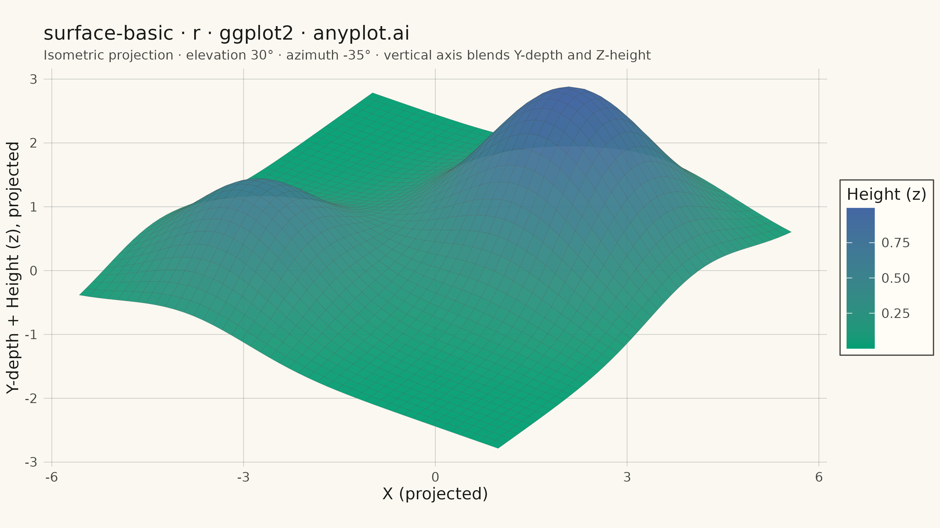
A 3D surface plot visualizes a function of two variables as a continuous surface in three-dimensional space. The height (z-axis) represents the function value at each (x, y) point, with color encoding the same information to enhance depth perception. This visualization is ideal for understanding mathematical functions, terrain data, and response surfaces where the relationship between two inputs and one output needs to be explored.
#' anyplot.ai
#' surface-basic: Basic 3D Surface Plot
#' Library: ggplot2 3.5.1 | R 4.4.1
#' Quality: 85/100 | Created: 2026-09-10
# anyplot.ai
# surface-basic: Basic 3D Surface Plot
# Library: ggplot2 | R
#
# ggplot2 has no native 3D device (no wireframe/surface geom), so the surface
# is rendered as a hand-projected mesh: rotate the (x, y, z) grid by a fixed
# elevation/azimuth, project it onto the 2D canvas, then draw one
# depth-sorted geom_polygon quad per grid cell (a painter's-algorithm mesh).
# Height is encoded twice — via the visual elevation of each quad and via its
# fill color — for redundant, colorblind-safe readability.

library(ggplot2)
library(dplyr)
library(ragg)

set.seed(42)

# --- Theme tokens -------------------------------------------------------------
THEME       <- Sys.getenv("ANYPLOT_THEME", "light")
PAGE_BG     <- if (THEME == "light") "#FAF8F1" else "#1A1A17"
ELEVATED_BG <- if (THEME == "light") "#FFFDF6" else "#242420"
INK         <- if (THEME == "light") "#1A1A17" else "#F0EFE8"
INK_SOFT    <- if (THEME == "light") "#4A4A44" else "#B8B7B0"

# --- Data: bimodal Gaussian response surface ----------------------------------
# z = f(x, y) over a 45x45 grid, e.g. a yield surface from two process
# settings — one dominant optimum plus a smaller secondary optimum.
n <- 45
x_vals <- seq(-4, 4, length.out = n)
y_vals <- seq(-4, 4, length.out = n)

X <- outer(y_vals, x_vals, function(y, x) x)
Y <- outer(y_vals, x_vals, function(y, x) y)
Z <- exp(-((X - 1.5)^2 + (Y - 1.5)^2) / 4) +
  0.6 * exp(-((X + 2)^2 + (Y + 2)^2) / 3)

# --- 3D -> 2D isometric projection ---------------------------------------------
elev <- 30 * pi / 180
azim <- -35 * pi / 180
z_scale <- 3 # visually amplify height relative to the x/y spatial extent

X_rot <- X * cos(azim) - Y * sin(azim)
Y_rot <- X * sin(azim) + Y * cos(azim)
Z_vis <- Z * z_scale

X_proj <- X_rot
Y_proj <- Y_rot * sin(elev) + Z_vis * cos(elev)

# One quad per grid cell: its 4 projected corners, mean height (fill) and
# mean depth (paint order — farthest cells first so nearer ones draw on top).
quads <- vector("list", (n - 1) * (n - 1))
k <- 1
for (i in 1:(n - 1)) {
  for (j in 1:(n - 1)) {
    quads[[k]] <- list(
      x = c(X_proj[i, j], X_proj[i, j + 1], X_proj[i + 1, j + 1], X_proj[i + 1, j]),
      y = c(Y_proj[i, j], Y_proj[i, j + 1], Y_proj[i + 1, j + 1], Y_proj[i + 1, j]),
      z = mean(c(Z[i, j], Z[i, j + 1], Z[i + 1, j + 1], Z[i + 1, j])),
      depth = mean(c(Y_rot[i, j], Y_rot[i, j + 1], Y_rot[i + 1, j + 1], Y_rot[i + 1, j]))
    )
    k <- k + 1
  }
}
quads <- quads[order(-vapply(quads, function(q) q$depth, numeric(1)))]

mesh_df <- bind_rows(lapply(seq_along(quads), function(g) {
  q <- quads[[g]]
  tibble::tibble(x = q$x, y = q$y, z = q$z, group = g)
}))

# --- Plot ----------------------------------------------------------------------
p <- ggplot(mesh_df, aes(x = x, y = y, group = group, fill = z)) +
  geom_polygon(color = adjustcolor(INK_SOFT, alpha.f = 0.45), linewidth = 0.07, alpha = 0.95) +
  scale_fill_gradient(low = "#009E73", high = "#4467A3", name = "Height (z)") +
  coord_fixed() +
  labs(
    title = "surface-basic · r · ggplot2 · anyplot.ai",
    subtitle = "Isometric projection · elevation 30° · azimuth -35° · vertical axis blends Y-depth and Z-height",
    x = "X (projected)",
    y = "Y-depth + Height (z), projected"
  ) +
  theme_minimal(base_size = 8) +
  theme(
    plot.background = element_rect(fill = PAGE_BG, color = PAGE_BG),
    panel.background = element_rect(fill = PAGE_BG, color = NA),
    panel.grid.major = element_line(color = adjustcolor(INK, alpha.f = 0.2), linewidth = 0.2),
    panel.grid.minor = element_blank(),
    axis.ticks = element_blank(),
    axis.line = element_blank(),
    axis.title = element_text(color = INK, size = 10),
    axis.text = element_text(color = INK_SOFT, size = 8),
    plot.title = element_text(color = INK, size = 12),
    plot.subtitle = element_text(color = INK_SOFT, size = 8),
    legend.background = element_rect(fill = ELEVATED_BG, color = INK_SOFT),
    legend.text = element_text(color = INK_SOFT, size = 8),
    legend.title = element_text(color = INK, size = 10)
  )

# --- Save -----------------------------------------------------------------------
ggsave(
  filename = sprintf("plot-%s.png", THEME),
  plot = p,
  device = ragg::agg_png,
  width = 8,
  height = 4.5,
  units = "in",
  dpi = 400
)
Runnable source as JSON, for any HTTP client: https://api.anyplot.ai/specs/surface-basic/ggplot2/code. Any spec id and library id listed in llms-full.txt fit the same URL shape; every URL below is complete and callable.
{
  "spec_id": "surface-basic",
  "language": "r",
  "library": "ggplot2",
  "page": "https://anyplot.ai/surface-basic/r/ggplot2",
  "hub": "https://anyplot.ai/surface-basic",
  "code_json": "https://api.anyplot.ai/specs/surface-basic/ggplot2/code",
  "spec_json": "https://api.anyplot.ai/specs/surface-basic",
  "render_light_png": "https://storage.googleapis.com/anyplot-images/plots/surface-basic/r/ggplot2/plot-light.png",
  "render_dark_png": "https://storage.googleapis.com/anyplot-images/plots/surface-basic/r/ggplot2/plot-dark.png",
  "quality_score": 85.0,
  "license": "MIT",
  "guide": "https://anyplot.ai/llms.txt"
}
Part of Basic 3D Surface Plot on anyplot.ai.