The same plot in 14 other libraries — Python: Altair, Bokeh, lets-plot, Matplotlib, Plotly, plotnine, Pygal, Seaborn; R: ggplot2; JavaScript: Chart.js, D3.js, Apache ECharts, Highcharts, MUI X Charts. Compare all 15 side by side: Basic Alluvial Diagram in Python, R, Julia and JavaScript.
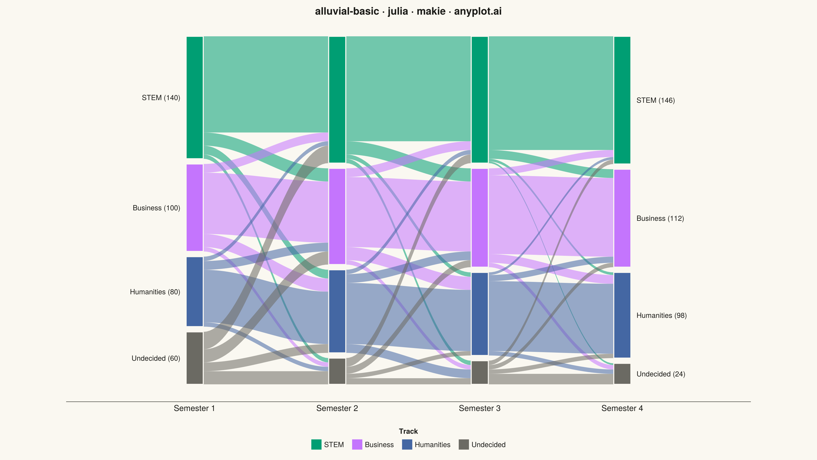
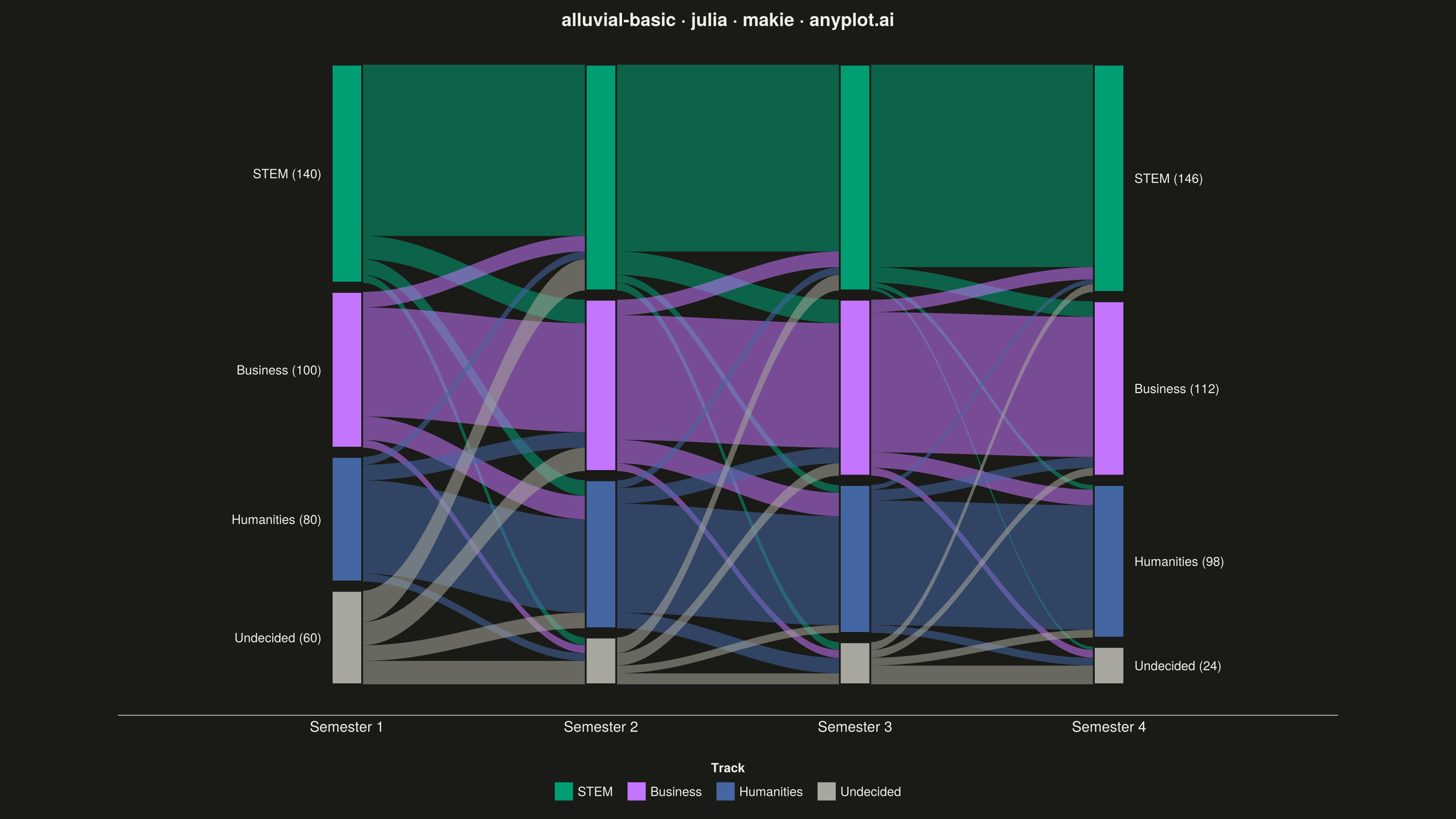
An alluvial diagram visualizes how entities flow or transition between discrete categories across multiple time points or ordered stages. Unlike general Sankey diagrams, alluvial diagrams enforce strict vertical ordering where each column represents a specific time step or category dimension. Bands connect related segments to show how proportions shift over time, making it ideal for tracking structural changes, migrations, and transitions in categorical data.
# anyplot.ai
# alluvial-basic: Basic Alluvial Diagram
# Library: makie 0.21.9 | Julia 1.11.9
# Quality: 90/100 | Created: 2026-09-02

using CairoMakie
using Colors

# --- Theme tokens -------------------------------------------------------------
const THEME     = get(ENV, "ANYPLOT_THEME", "light")
const PAGE_BG   = THEME == "light" ? colorant"#FAF8F1" : colorant"#1A1A17"
const INK       = THEME == "light" ? colorant"#1A1A17" : colorant"#F0EFE8"
const INK_SOFT  = THEME == "light" ? colorant"#4A4A44" : colorant"#B8B7B0"
const INK_MUTED = THEME == "light" ? colorant"#6B6A63" : colorant"#A8A79F"
const IMPRINT_PALETTE = [
    colorant"#009E73",  # 1 — brand green
    colorant"#C475FD",  # 2 — lavender
    colorant"#4467A3",  # 3 — blue
]

# --- Data: academic track transitions across four semesters -------------------
# Undecided is mapped to the theme-adaptive "muted" semantic anchor rather than
# a categorical slot — it literally represents a neutral / uncommitted state.
categories      = ["STEM", "Business", "Humanities", "Undecided"]
category_colors = [IMPRINT_PALETTE[1], IMPRINT_PALETTE[2], IMPRINT_PALETTE[3], INK_MUTED]
time_labels     = ["Semester 1", "Semester 2", "Semester 3", "Semester 4"]

nt   = length(time_labels)
ncat = length(categories)

# values[t, k] — enrolled students in category k at time point t
values = Float64[
    140 100  80 60
    145 110  95 30
    145 113  95 27
    146 112  98 24
]

# flows[t][i, j] — students moving from category i (at time t) to category j (at time t+1)
flows = [
    Float64[110 15 10  5; 10 70 15  5;  5 10 60  5; 20 15 10 15],
    Float64[120 15  5  5; 10 80 15  5;  5 10 70 10; 10  8  5  7],
    Float64[130 10  3  2;  8 90 10  5;  3  7 80  5;  5  5  5 12],
]

# --- Layout: stack each column's categories top-to-bottom with a fixed gap ---
gap = 6.0
node_top = zeros(Float64, nt, ncat)
node_bot = zeros(Float64, nt, ncat)
for t in 1:nt
    cursor = 0.0
    for k in 1:ncat
        node_top[t, k] = cursor
        node_bot[t, k] = cursor - values[t, k]
        cursor = node_bot[t, k] - gap
    end
end

node_halfwidth = 0.06
npts = 40

# --- Plot -----------------------------------------------------------------
fig = Figure(
    resolution      = (1600, 900),
    fontsize        = 14,
    backgroundcolor = PAGE_BG,
    figure_padding  = (130, 130, 10, 10),
)

ax = Axis(
    fig[1, 1];
    title              = "alluvial-basic · julia · makie · anyplot.ai",
    titlesize          = 20,
    titlecolor         = INK,
    xticks             = (1:nt, time_labels),
    xticklabelsize     = 16,
    xticklabelcolor    = INK,
    xticksvisible      = false,
    yticksvisible      = false,
    yticklabelsvisible = false,
    ylabelvisible      = false,
    xgridvisible       = false,
    ygridvisible       = false,
    topspinevisible    = false,
    rightspinevisible  = false,
    leftspinevisible   = false,
    bottomspinecolor   = INK_SOFT,
    backgroundcolor    = PAGE_BG,
)

# Flow bands (drawn first, sit beneath the nodes). Sub-segments within a source
# node are ordered by destination category, and within a destination node by
# source category, so bands never cross their own siblings.
for t in 1:(nt - 1)
    out_cursor = copy(node_top[t, :])
    in_cursor  = copy(node_top[t + 1, :])
    for i in 1:ncat, j in 1:ncat
        f = flows[t][i, j]
        f <= 0 && continue

        src_top = out_cursor[i]
        src_bot = src_top - f
        out_cursor[i] = src_bot

        dst_top = in_cursor[j]
        dst_bot = dst_top - f
        in_cursor[j] = dst_bot

        x_left  = t + node_halfwidth
        x_right = (t + 1) - node_halfwidth
        xs = range(x_left, x_right, length = npts)
        ease = [(1 - cos(pi * (x - x_left) / (x_right - x_left))) / 2 for x in xs]
        ys_top = src_top .+ (dst_top - src_top) .* ease
        ys_bot = src_bot .+ (dst_bot - src_bot) .* ease

        band_pts = vcat(Point2f.(xs, ys_top), Point2f.(reverse(xs), reverse(ys_bot)))
        poly!(ax, band_pts; color = (category_colors[i], 0.55), strokewidth = 0)
    end
end

# Nodes (stacked category blocks per time point)
for t in 1:nt, k in 1:ncat
    corners = Point2f[
        (t - node_halfwidth, node_top[t, k]),
        (t + node_halfwidth, node_top[t, k]),
        (t + node_halfwidth, node_bot[t, k]),
        (t - node_halfwidth, node_bot[t, k]),
    ]
    poly!(ax, corners; color = category_colors[k], strokecolor = PAGE_BG, strokewidth = 2)
end

# Category labels at the first and last column, with enrollment counts
for k in 1:ncat
    y_first = (node_top[1, k] + node_bot[1, k]) / 2
    text!(ax, 1 - node_halfwidth - 0.04, y_first;
          text = "$(categories[k]) ($(Int(values[1, k])))",
          align = (:right, :center), color = INK, fontsize = 14)

    y_last = (node_top[nt, k] + node_bot[nt, k]) / 2
    text!(ax, nt + node_halfwidth + 0.04, y_last;
          text = "$(categories[k]) ($(Int(values[nt, k])))",
          align = (:left, :center), color = INK, fontsize = 14)
end

xlims!(ax, 1 - 0.9, nt + 0.9)

legend_elems = [PolyElement(color = c) for c in category_colors]
Legend(
    fig[2, 1], legend_elems, categories, "Track";
    orientation = :horizontal, tellwidth = false, framevisible = false,
    labelcolor = INK, titlecolor = INK,
)
rowsize!(fig.layout, 2, Relative(0.08))

# --- Save -----------------------------------------------------------------
save("plot-$(THEME).png", fig; px_per_unit = 2)
Runnable source as JSON, for any HTTP client: https://api.anyplot.ai/specs/alluvial-basic/makie/code. Any spec id and library id listed in llms-full.txt fit the same URL shape; every URL below is complete and callable.
{
  "spec_id": "alluvial-basic",
  "language": "julia",
  "library": "makie",
  "page": "https://anyplot.ai/alluvial-basic/julia/makie",
  "hub": "https://anyplot.ai/alluvial-basic",
  "code_json": "https://api.anyplot.ai/specs/alluvial-basic/makie/code",
  "spec_json": "https://api.anyplot.ai/specs/alluvial-basic",
  "render_light_png": "https://storage.googleapis.com/anyplot-images/plots/alluvial-basic/julia/makie/plot-light.png",
  "render_dark_png": "https://storage.googleapis.com/anyplot-images/plots/alluvial-basic/julia/makie/plot-dark.png",
  "quality_score": 90.0,
  "license": "MIT",
  "guide": "https://anyplot.ai/llms.txt"
}
Part of Basic Alluvial Diagram on anyplot.ai.