The same plot in 14 other libraries — Python: Altair, Bokeh, lets-plot, Matplotlib, Plotly, plotnine, Pygal, Seaborn; Julia: Makie.jl; JavaScript: Chart.js, D3.js, Apache ECharts, Highcharts, MUI X Charts. Compare all 15 side by side: Basic Alluvial Diagram in Python, R, Julia and JavaScript.
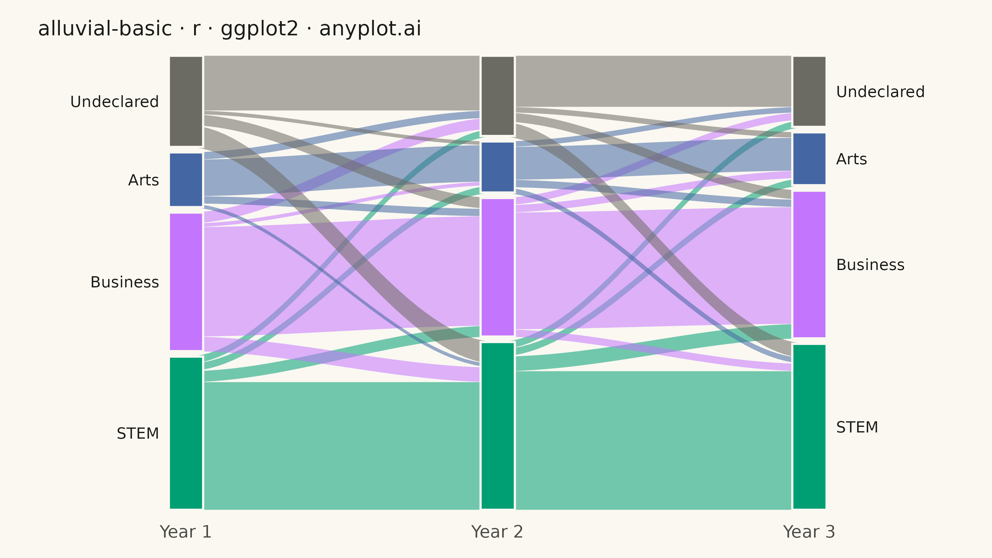
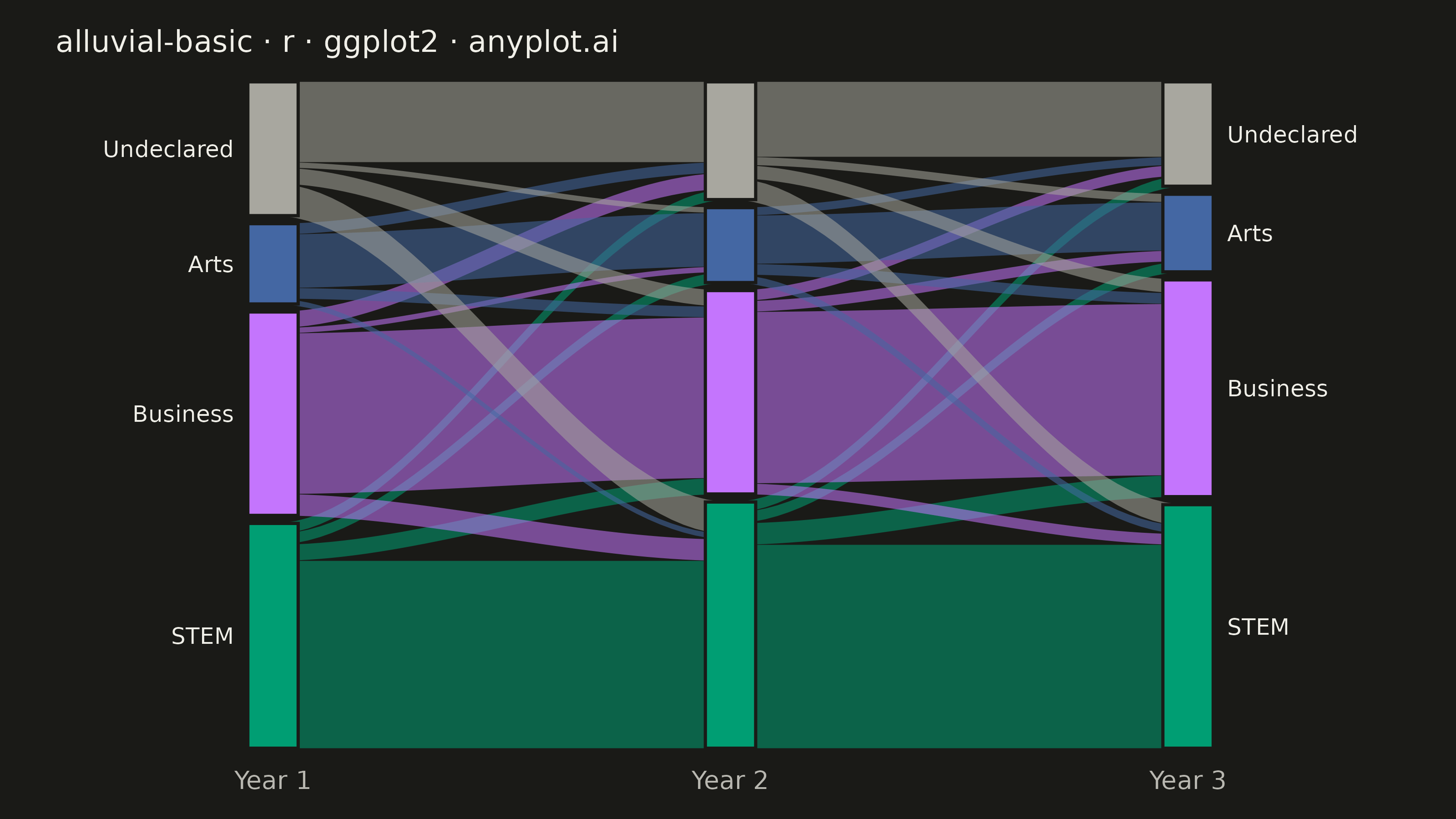
An alluvial diagram visualizes how entities flow or transition between discrete categories across multiple time points or ordered stages. Unlike general Sankey diagrams, alluvial diagrams enforce strict vertical ordering where each column represents a specific time step or category dimension. Bands connect related segments to show how proportions shift over time, making it ideal for tracking structural changes, migrations, and transitions in categorical data.
#' anyplot.ai
#' alluvial-basic: Basic Alluvial Diagram
#' Library: ggplot2 3.5.1 | R 4.4.1
#' Quality: 88/100 | Created: 2026-09-02

library(ggplot2)
library(dplyr)
library(ragg)

set.seed(42)

# --- Theme tokens -------------------------------------------------------
THEME     <- Sys.getenv("ANYPLOT_THEME", "light")
PAGE_BG   <- if (THEME == "light") "#FAF8F1" else "#1A1A17"
INK       <- if (THEME == "light") "#1A1A17" else "#F0EFE8"
INK_SOFT  <- if (THEME == "light") "#4A4A44" else "#B8B7B0"
INK_MUTED <- if (THEME == "light") "#6B6A63" else "#A8A79F"

# Imprint palette (see prompts/default-style-guide.md "Categorical Palette")
IMPRINT_PALETTE <- c("#009E73", "#C475FD", "#4467A3", "#BD8233",
                     "#AE3030", "#2ABCCD", "#954477", "#99B314")

CATEGORY_ORDER <- c("STEM", "Business", "Arts", "Undeclared")
CATEGORY_COLORS <- c(
  STEM       = IMPRINT_PALETTE[1],
  Business   = IMPRINT_PALETTE[2],
  Arts       = IMPRINT_PALETTE[3],
  Undeclared = INK_MUTED  # semantic anchor: undecided majors read as "other"
)
STAGE_LABELS <- c("Year 1", "Year 2", "Year 3")
NODE_WIDTH   <- 0.055
GAP          <- 15  # visual spacing between stacked categories at a stage

# --- Data: student counts transitioning between academic tracks --------
# ggplot2 has no native Sankey/alluvial geom (ggalluvial is not installed in
# this environment) — the bands below are built from first principles with
# stacked node ranges and a smoothstep interpolation, using only geom_ribbon
# and geom_rect, both native ggplot2 geoms.
flows <- tibble::tribble(
  ~stage_from, ~stage_to, ~cat_from,    ~cat_to,      ~value,
  1, 2, "STEM",       "STEM",       350,
  1, 2, "STEM",       "Business",    30,
  1, 2, "STEM",       "Arts",        20,
  1, 2, "STEM",       "Undeclared",  20,
  1, 2, "Business",   "STEM",        40,
  1, 2, "Business",   "Business",   300,
  1, 2, "Business",   "Arts",        10,
  1, 2, "Business",   "Undeclared",  30,
  1, 2, "Arts",       "STEM",        10,
  1, 2, "Arts",       "Business",    20,
  1, 2, "Arts",       "Arts",       100,
  1, 2, "Arts",       "Undeclared",  20,
  1, 2, "Undeclared", "STEM",        60,
  1, 2, "Undeclared", "Business",    30,
  1, 2, "Undeclared", "Arts",        10,
  1, 2, "Undeclared", "Undeclared", 150,
  2, 3, "STEM",       "STEM",       380,
  2, 3, "STEM",       "Business",    40,
  2, 3, "STEM",       "Arts",        20,
  2, 3, "STEM",       "Undeclared",  20,
  2, 3, "Business",   "STEM",        20,
  2, 3, "Business",   "Business",   320,
  2, 3, "Business",   "Arts",        20,
  2, 3, "Business",   "Undeclared",  20,
  2, 3, "Arts",       "STEM",        15,
  2, 3, "Arts",       "Business",    20,
  2, 3, "Arts",       "Arts",        90,
  2, 3, "Arts",       "Undeclared",  15,
  2, 3, "Undeclared", "STEM",        40,
  2, 3, "Undeclared", "Business",    25,
  2, 3, "Undeclared", "Arts",        15,
  2, 3, "Undeclared", "Undeclared", 140
) %>%
  mutate(row_id = row_number())

# --- Node totals & stacked y-ranges per stage (fixed category order) ----
node_totals <- bind_rows(
  flows %>% group_by(stage = stage_from, category = cat_from) %>%
    summarise(total = sum(value), .groups = "drop"),
  flows %>% filter(stage_to == max(stage_to)) %>%
    group_by(stage = stage_to, category = cat_to) %>%
    summarise(total = sum(value), .groups = "drop")
) %>%
  mutate(category = factor(category, levels = CATEGORY_ORDER)) %>%
  arrange(stage, category) %>%
  group_by(stage) %>%
  mutate(
    ymax = cumsum(total) + GAP * (row_number() - 1),
    ymin = ymax - total
  ) %>%
  ungroup()

# --- Stack outgoing / incoming flows inside each node --------------------
out_offsets <- flows %>%
  mutate(cat_to_f = factor(cat_to, levels = CATEGORY_ORDER)) %>%
  group_by(stage_from, cat_from) %>%
  arrange(cat_to_f, .by_group = TRUE) %>%
  mutate(y1_local = cumsum(value), y0_local = y1_local - value) %>%
  ungroup() %>%
  left_join(
    node_totals %>% transmute(stage_from = stage, cat_from = as.character(category), node_ymin = ymin),
    by = c("stage_from", "cat_from")
  ) %>%
  transmute(row_id, y0_from = node_ymin + y0_local, y1_from = node_ymin + y1_local)

in_offsets <- flows %>%
  mutate(cat_from_f = factor(cat_from, levels = CATEGORY_ORDER)) %>%
  group_by(stage_to, cat_to) %>%
  arrange(cat_from_f, .by_group = TRUE) %>%
  mutate(y1_local = cumsum(value), y0_local = y1_local - value) %>%
  ungroup() %>%
  left_join(
    node_totals %>% transmute(stage_to = stage, cat_to = as.character(category), node_ymin = ymin),
    by = c("stage_to", "cat_to")
  ) %>%
  transmute(row_id, y0_to = node_ymin + y0_local, y1_to = node_ymin + y1_local)

flows_full <- flows %>%
  left_join(out_offsets, by = "row_id") %>%
  left_join(in_offsets, by = "row_id")

# --- Smooth alluvial bands via smoothstep interpolation ------------------
smooth_band <- function(x_from, x_to, y0_from, y1_from, y0_to, y1_to, row_id, cat_from, n = 40) {
  t <- seq(0, 1, length.out = n)
  w <- t^2 * (3 - 2 * t)  # smoothstep S-curve
  tibble::tibble(
    row_id   = row_id,
    cat_from = cat_from,
    x        = x_from + t * (x_to - x_from),
    ymin     = y0_from + w * (y0_to - y0_from),
    ymax     = y1_from + w * (y1_to - y1_from)
  )
}

bands <- bind_rows(lapply(seq_len(nrow(flows_full)), function(i) {
  r <- flows_full[i, ]
  smooth_band(r$stage_from, r$stage_to, r$y0_from, r$y1_from, r$y0_to, r$y1_to, r$row_id, r$cat_from)
}))
bands$cat_from <- factor(bands$cat_from, levels = CATEGORY_ORDER)

# --- Node labels (category name shown at the first & last stage only) ----
node_labels <- node_totals %>%
  filter(stage %in% range(stage)) %>%
  mutate(
    y     = (ymin + ymax) / 2,
    x     = if_else(stage == min(stage), stage - NODE_WIDTH - 0.03, stage + NODE_WIDTH + 0.03),
    hjust = if_else(stage == min(stage), 1, 0)
  )

# --- Mini legend (covers the middle stage, where nodes have no free space
# alongside them for direct labels since ribbons flank both sides) ----------
max_y <- max(node_totals$ymax)
legend_y <- max_y * 1.09
legend_data <- tibble::tibble(
  category = factor(CATEGORY_ORDER, levels = CATEGORY_ORDER),
  x        = 2 + seq(-0.42, 0.42, length.out = length(CATEGORY_ORDER)),
  y        = legend_y
)

# --- Plot ------------------------------------------------------------------
p <- ggplot() +
  geom_ribbon(
    data = bands,
    aes(x = x, ymin = ymin, ymax = ymax, group = row_id, fill = cat_from),
    color = INK, linewidth = 0.15, alpha = 0.45
  ) +
  geom_rect(
    data = node_totals,
    aes(xmin = stage - NODE_WIDTH, xmax = stage + NODE_WIDTH,
        ymin = ymin, ymax = ymax, fill = category),
    color = PAGE_BG, linewidth = 0.6
  ) +
  geom_text(
    data = node_labels,
    aes(x = x, y = y, label = category, hjust = hjust),
    size = 4, color = INK
  ) +
  geom_point(
    data = legend_data,
    aes(x = x, y = y),
    color = CATEGORY_COLORS[as.character(legend_data$category)],
    shape = 15, size = 3.5
  ) +
  geom_text(
    data = legend_data,
    aes(x = x + 0.06, y = y, label = category),
    size = 2.9, color = INK_SOFT, hjust = 0, vjust = 0.4
  ) +
  scale_fill_manual(values = CATEGORY_COLORS, guide = "none") +
  scale_x_continuous(
    breaks = seq_along(STAGE_LABELS), labels = STAGE_LABELS,
    expand = expansion(mult = c(0.18, 0.18))
  ) +
  scale_y_continuous(expand = expansion(mult = c(0.02, 0.1))) +
  labs(
    title = "alluvial-basic · r · ggplot2 · anyplot.ai",
    x = NULL, y = NULL
  ) +
  theme_minimal(base_size = 8) +
  theme(
    plot.background  = element_rect(fill = PAGE_BG, color = PAGE_BG),
    panel.background = element_rect(fill = PAGE_BG, color = NA),
    panel.grid       = element_blank(),
    axis.title       = element_blank(),
    axis.text.y      = element_blank(),
    axis.ticks       = element_blank(),
    axis.text.x      = element_text(color = INK_SOFT, size = 10),
    plot.title       = element_text(color = INK, size = 12),
    plot.margin      = margin(12, 20, 10, 20)
  )

# --- Save --------------------------------------------------------------------
ggsave(
  filename = sprintf("plot-%s.png", THEME),
  plot     = p,
  device   = ragg::agg_png,
  width    = 8,
  height   = 4.5,
  units    = "in",
  dpi      = 400
)
Runnable source as JSON, for any HTTP client: https://api.anyplot.ai/specs/alluvial-basic/ggplot2/code. Any spec id and library id listed in llms-full.txt fit the same URL shape; every URL below is complete and callable.
{
  "spec_id": "alluvial-basic",
  "language": "r",
  "library": "ggplot2",
  "page": "https://anyplot.ai/alluvial-basic/r/ggplot2",
  "hub": "https://anyplot.ai/alluvial-basic",
  "code_json": "https://api.anyplot.ai/specs/alluvial-basic/ggplot2/code",
  "spec_json": "https://api.anyplot.ai/specs/alluvial-basic",
  "render_light_png": "https://storage.googleapis.com/anyplot-images/plots/alluvial-basic/r/ggplot2/plot-light.png",
  "render_dark_png": "https://storage.googleapis.com/anyplot-images/plots/alluvial-basic/r/ggplot2/plot-dark.png",
  "quality_score": 88.0,
  "license": "MIT",
  "guide": "https://anyplot.ai/llms.txt"
}
Part of Basic Alluvial Diagram on anyplot.ai.