The same plot in 14 other libraries — JavaScript: Chart.js, Apache ECharts, Highcharts, MUI X Charts; Python: Altair, Bokeh, lets-plot, Matplotlib, Plotly, plotnine, Pygal, Seaborn; R: ggplot2; Julia: Makie.jl. Compare all 15 side by side: Stacked Area Chart with Confidence Bands in Python, R, Julia and JavaScript.
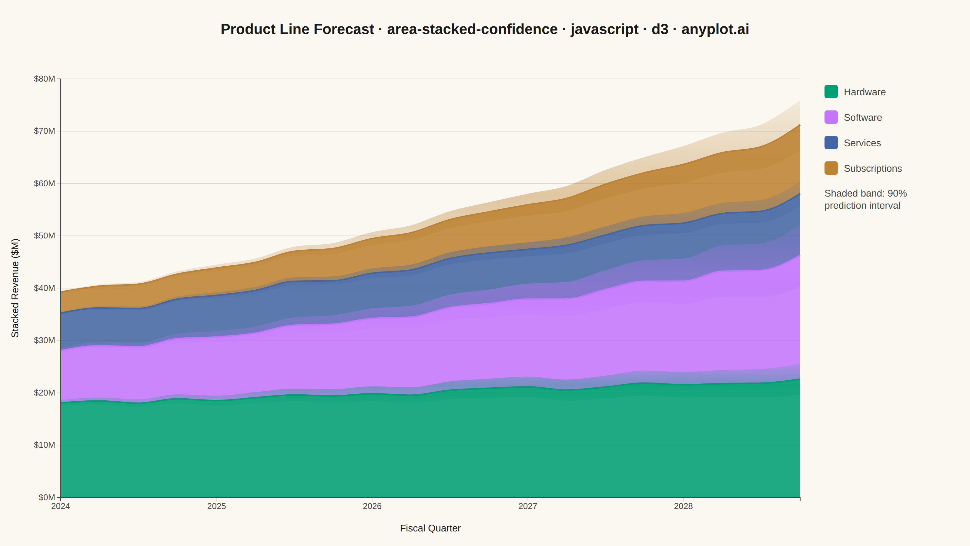
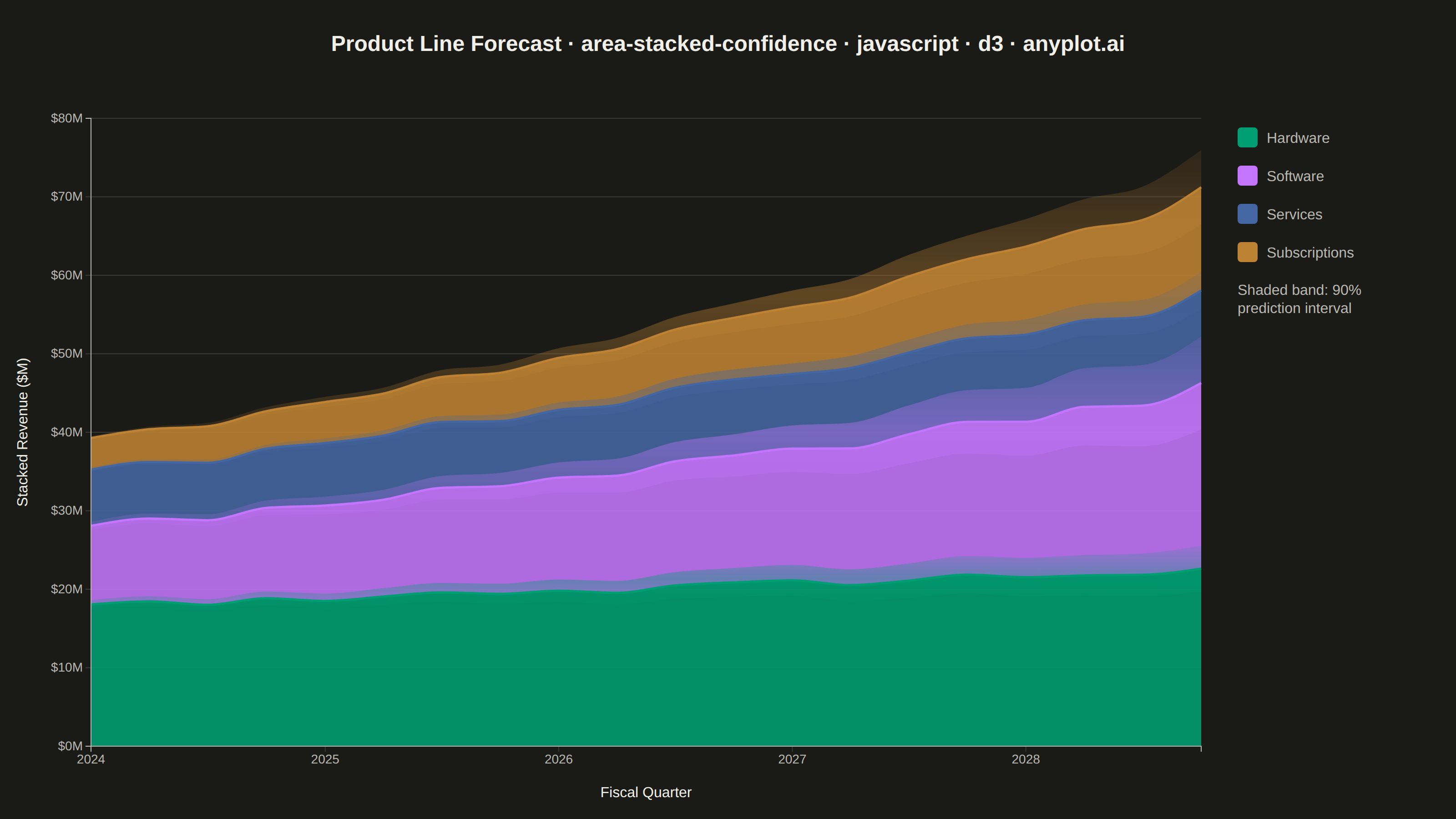
A stacked area chart that displays multiple data series as cumulative areas, with each series surrounded by uncertainty or confidence bands. This visualization combines the composition insight of stacked areas with the statistical rigor of confidence intervals, making it ideal for showing how parts contribute to a whole while simultaneously communicating uncertainty in each component. The bands reveal where estimates are precise versus uncertain across the stacked series.
// anyplot.ai
// area-stacked-confidence: Stacked Area Chart with Confidence Bands
// Library: d3 7.9.0 | JavaScript 22.23.2
// Quality: 94/100 | Created: 2026-08-26

const t = window.ANYPLOT_TOKENS;
const { width, height } = window.ANYPLOT_SIZE;

// --- Deterministic PRNG (fixed-seed LCG — no seeded RNG in the browser) ----
let seed = 42;
function rand() {
  seed = (seed * 1103515245 + 12345) & 0x7fffffff;
  return seed / 0x7fffffff;
}

// --- Data: quarterly revenue forecast by product line, with 90% prediction
//     intervals that widen further into the forecast horizon — the newer,
//     faster-growing lines (Subscriptions) are inherently harder to forecast
//     than the mature ones (Hardware), so each series gets its own band-
//     growth rate rather than a shared fractional curve -------------------
const productLines = ["Hardware", "Software", "Services", "Subscriptions"];
const baseRevenue = [18, 10, 7, 4];
const growthPerQuarter = [0.012, 0.045, 0.028, 0.065];
const bandBaseFrac = [0.03, 0.05, 0.04, 0.06];
const bandGrowthFrac = [0.1, 0.2, 0.16, 0.3];
const nQuarters = 20;
const dates = d3.range(nQuarters).map((i) => new Date(2024, i * 3, 1));
const keys = productLines.map((_, s) => `y${s}`);

const data = dates.map((date, i) => {
  const row = { date };
  productLines.forEach((_, s) => {
    const key = keys[s];
    const wobble = 1 + (rand() - 0.5) * 0.05;
    row[key] = baseRevenue[s] * Math.pow(1 + growthPerQuarter[s], i) * wobble;
    row[`${key}_band`] = bandBaseFrac[s] + (i / (nQuarters - 1)) * bandGrowthFrac[s];
  });
  return row;
});

// --- Stack central values; derive confidence bands from the same stack
//     order so each layer's band sits atop its own cumulative baseline ----
const stacked = d3.stack().keys(keys)(data);

const bands = stacked.map((layer) =>
  layer.map((point, j) => {
    const key = layer.key;
    const y0 = point[0];
    const central = data[j][key];
    const frac = data[j][`${key}_band`];
    return { date: data[j].date, low: y0 + central * (1 - frac), high: y0 + central * (1 + frac) };
  }),
);

// --- Layout -----------------------------------------------------------------
const margin = { top: 130, right: 280, bottom: 80, left: 100 };
const iw = width - margin.left - margin.right;
const ih = height - margin.top - margin.bottom;

const x = d3.scaleTime().domain(d3.extent(dates)).range([0, iw]);
const yMax = d3.max(bands[bands.length - 1], (d) => d.high);
const y = d3.scaleLinear().domain([0, yMax]).nice().range([ih, 0]);

// --- SVG mount ----------------------------------------------------------------
const svg = d3.select("#container").append("svg").attr("width", width).attr("height", height);
const g = svg.append("g").attr("transform", `translate(${margin.left},${margin.top})`);

// --- Gridlines (y-axis only) -------------------------------------------------
g.append("g")
  .attr("class", "grid")
  .call(d3.axisLeft(y).ticks(6).tickSize(-iw).tickFormat(""))
  .call((gr) => gr.select(".domain").remove())
  .call((gr) => gr.selectAll("line").attr("stroke", t.grid));

// --- Areas: shape generators --------------------------------------------------
const areaCentral = d3
  .area()
  .x((d) => x(d.data.date))
  .y0((d) => y(d[0]))
  .y1((d) => y(d[1]))
  .curve(d3.curveMonotoneX);

const areaBand = d3
  .area()
  .x((d) => x(d.date))
  .y0((d) => y(d.low))
  .y1((d) => y(d.high))
  .curve(d3.curveMonotoneX);

const lineTop = d3
  .line()
  .x((d) => x(d.data.date))
  .y((d) => y(d[1]))
  .curve(d3.curveMonotoneX);

// Per-series vertical gradient for the confidence bands: opacity peaks at the
// midpoint (close to each column's central estimate, since bands are built
// symmetric around it) and tapers toward the low/high edges — reads as a
// soft "cloud" of uncertainty rather than a flat tint.
const defs = svg.append("defs");
productLines.forEach((_, i) => {
  const gradient = defs
    .append("linearGradient")
    .attr("id", `band-gradient-${i}`)
    .attr("x1", "0")
    .attr("x2", "0")
    .attr("y1", "0")
    .attr("y2", "1");
  gradient.append("stop").attr("offset", "0%").attr("stop-color", t.palette[i]).attr("stop-opacity", 0.12);
  gradient.append("stop").attr("offset", "50%").attr("stop-color", t.palette[i]).attr("stop-opacity", 0.42);
  gradient.append("stop").attr("offset", "100%").attr("stop-color", t.palette[i]).attr("stop-opacity", 0.12);
});

// Stacked central areas first, translucent gradient bands on top (so a band
// bleeding past its series' own boundary blends into the neighbor, showing
// where the two series' uncertainty overlaps), then crisp boundary lines on
// top of both.
stacked.forEach((layer, i) => {
  g.append("path").datum(layer).attr("fill", t.palette[i]).attr("fill-opacity", 0.88).attr("d", areaCentral);
});
bands.forEach((band, i) => {
  g.append("path").datum(band).attr("fill", `url(#band-gradient-${i})`).attr("d", areaBand);
});
stacked.forEach((layer, i) => {
  g.append("path")
    .datum(layer)
    .attr("fill", "none")
    .attr("stroke", t.palette[i])
    .attr("stroke-width", 2.5)
    .attr("d", lineTop);
});

// --- Axes ---------------------------------------------------------------------
const xAxis = g
  .append("g")
  .attr("transform", `translate(0,${ih})`)
  .call(d3.axisBottom(x).ticks(d3.timeYear.every(1)).tickFormat(d3.timeFormat("%Y")));
xAxis.selectAll("text").attr("fill", t.inkSoft).style("font-size", "14px");
xAxis.selectAll("line").attr("stroke", t.grid);
xAxis.select(".domain").attr("stroke", t.inkSoft);

const yAxis = g.append("g").call(
  d3
    .axisLeft(y)
    .ticks(6)
    .tickFormat((d) => `$${d}M`),
);
yAxis.selectAll("text").attr("fill", t.inkSoft).style("font-size", "14px");
yAxis.selectAll("line").attr("stroke", t.grid);
yAxis.select(".domain").attr("stroke", t.inkSoft);

// --- Axis titles ----------------------------------------------------------------
g.append("text")
  .attr("x", iw / 2)
  .attr("y", ih + 56)
  .attr("text-anchor", "middle")
  .attr("fill", t.ink)
  .style("font-size", "16px")
  .text("Fiscal Quarter");

g.append("text")
  .attr("transform", "rotate(-90)")
  .attr("x", -ih / 2)
  .attr("y", -70)
  .attr("text-anchor", "middle")
  .attr("fill", t.ink)
  .style("font-size", "16px")
  .text("Stacked Revenue ($M)");

// --- Legend ---------------------------------------------------------------------
const legend = svg.append("g").attr("transform", `translate(${width - margin.right + 40},${margin.top + 10})`);
productLines.forEach((name, i) => {
  const row = legend.append("g").attr("transform", `translate(0,${i * 42})`);
  row.append("rect").attr("width", 22).attr("height", 22).attr("rx", 4).attr("fill", t.palette[i]);
  row
    .append("text")
    .attr("x", 32)
    .attr("y", 17)
    .attr("fill", t.inkSoft)
    .style("font-size", "16px")
    .text(name);
});
legend
  .append("text")
  .attr("x", 0)
  .attr("y", productLines.length * 42 + 16)
  .attr("fill", t.inkSoft)
  .style("font-size", "16px")
  .text("Shaded band: 90%")
  .append("tspan")
  .attr("x", 0)
  .attr("dy", 20)
  .text("prediction interval");

// --- Title ------------------------------------------------------------------
const title = "Product Line Forecast · area-stacked-confidence · javascript · d3 · anyplot.ai";
// Descriptive-prefixed titles run well past the 67-char mandated baseline; a
// strict linear shrink off the 22px default undershoots (reads at ~43% of
// canvas width). Scale off a taller 28px baseline instead, floored at 18px,
// so long titles stay prominent (~50-60% of width) without overflowing.
const titleFontSize = Math.max(18, Math.round(28 * (title.length > 67 ? 67 / title.length : 1)));
svg
  .append("text")
  .attr("x", width / 2)
  .attr("y", 56)
  .attr("text-anchor", "middle")
  .attr("fill", t.ink)
  .style("font-size", `${titleFontSize}px`)
  .style("font-weight", "600")
  .text(title);
Runnable source as JSON, for any HTTP client: https://api.anyplot.ai/specs/area-stacked-confidence/d3/code. Any spec id and library id listed in llms-full.txt fit the same URL shape; every URL below is complete and callable.
{
  "spec_id": "area-stacked-confidence",
  "language": "javascript",
  "library": "d3",
  "page": "https://anyplot.ai/area-stacked-confidence/javascript/d3",
  "hub": "https://anyplot.ai/area-stacked-confidence",
  "code_json": "https://api.anyplot.ai/specs/area-stacked-confidence/d3/code",
  "spec_json": "https://api.anyplot.ai/specs/area-stacked-confidence",
  "render_light_png": "https://storage.googleapis.com/anyplot-images/plots/area-stacked-confidence/javascript/d3/plot-light.png",
  "render_dark_png": "https://storage.googleapis.com/anyplot-images/plots/area-stacked-confidence/javascript/d3/plot-dark.png",
  "interactive_light_html": "https://storage.googleapis.com/anyplot-images/plots/area-stacked-confidence/javascript/d3/plot-light.html",
  "interactive_dark_html": "https://storage.googleapis.com/anyplot-images/plots/area-stacked-confidence/javascript/d3/plot-dark.html",
  "quality_score": 94.0,
  "license": "MIT",
  "guide": "https://anyplot.ai/llms.txt"
}
Part of Stacked Area Chart with Confidence Bands on anyplot.ai.