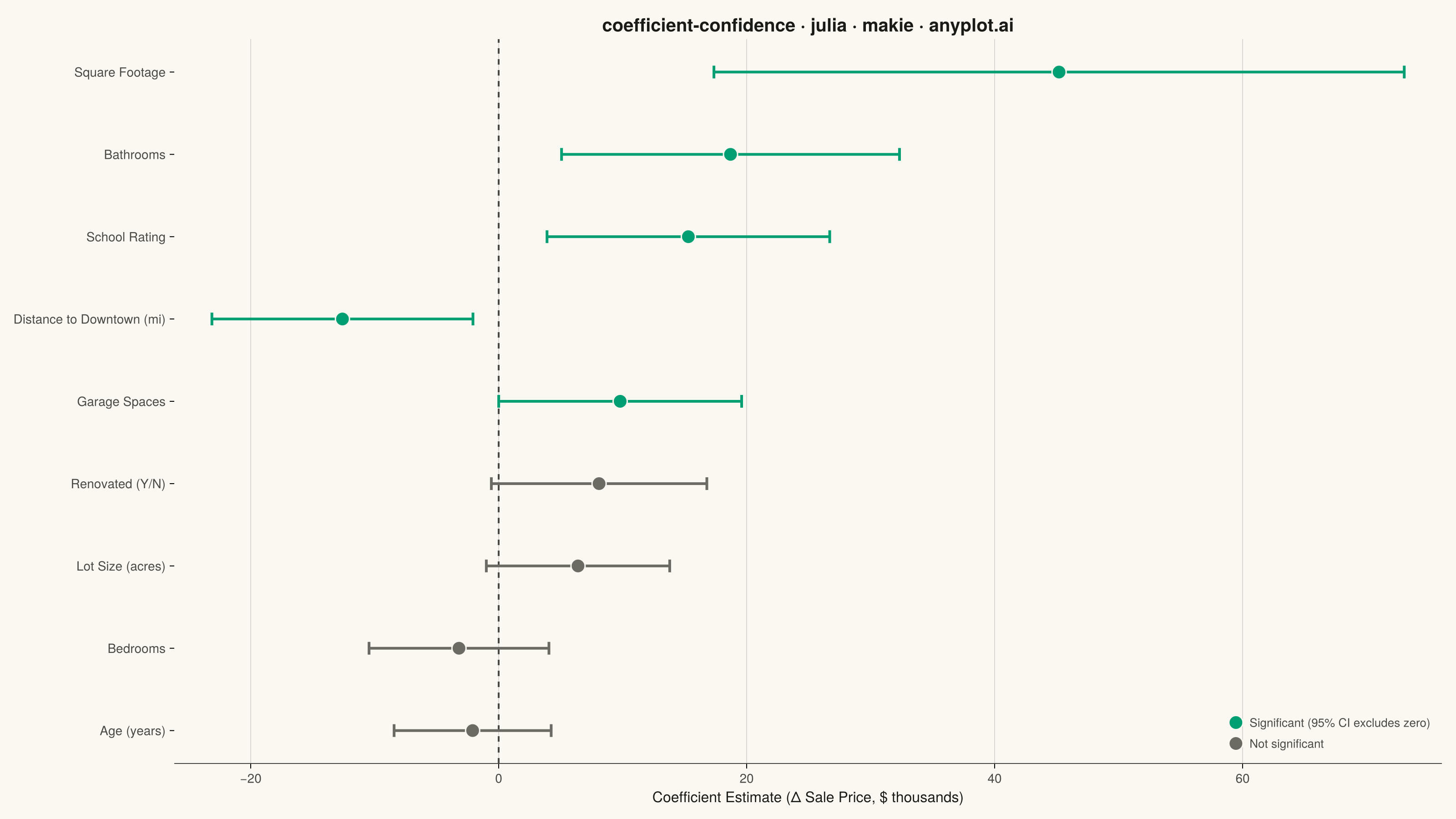
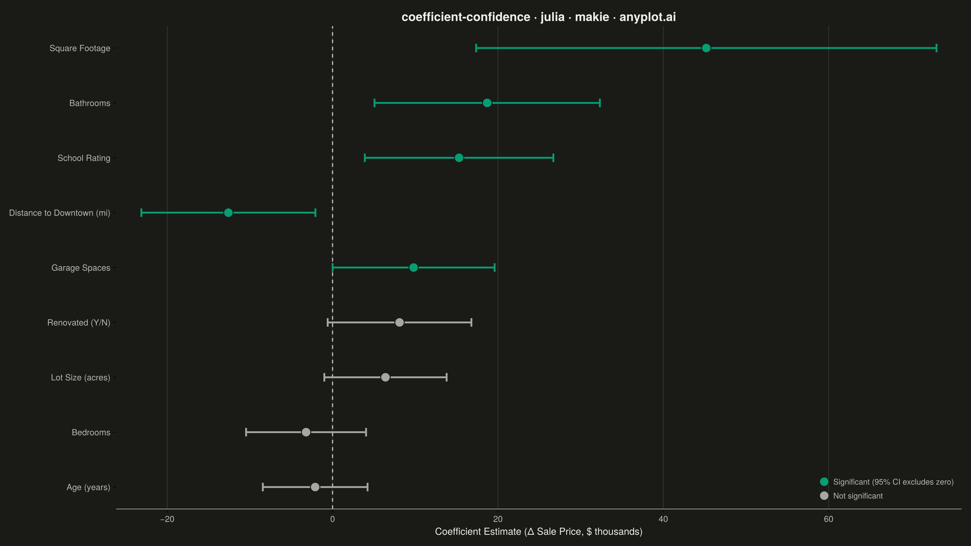
The same plot in 14 other libraries — Python: Altair, Bokeh, lets-plot, Matplotlib, Plotly, plotnine, Pygal, Seaborn; R: ggplot2; JavaScript: Chart.js, D3.js, Apache ECharts, Highcharts, MUI X Charts. Compare all 15 side by side: Coefficient Plot with Confidence Intervals in Python, R, Julia and JavaScript.
A coefficient plot displays regression coefficients as points positioned along a horizontal axis, with horizontal error bars showing confidence intervals. This visualization makes it easy to assess effect sizes and statistical significance - coefficients whose confidence intervals cross zero are not statistically significant. Typically used to summarize results from linear, logistic, or other regression models in a clear, publication-ready format.
# anyplot.ai
# coefficient-confidence: Coefficient Plot with Confidence Intervals
# Library: makie 0.21.9 | Julia 1.11.9
# Quality: 90/100 | Created: 2026-09-01

using CairoMakie
using Colors
using Random
using Printf

Random.seed!(42)

# Theme tokens (see prompts/default-style-guide.md "Background" + "Theme-adaptive Chrome")
THEME     = get(ENV, "ANYPLOT_THEME", "light")
PAGE_BG   = THEME == "light" ? colorant"#FAF8F1" : colorant"#1A1A17"
INK       = THEME == "light" ? colorant"#1A1A17" : colorant"#F0EFE8"
INK_SOFT  = THEME == "light" ? colorant"#4A4A44" : colorant"#B8B7B0"
INK_MUTED = THEME == "light" ? colorant"#6B6A63" : colorant"#A8A79F"
BRAND     = colorant"#009E73"  # Imprint palette position 1 — significant coefficients

# Data — coefficients from a multiple linear regression predicting housing sale
# price (thousands of USD), controlling for all other predictors.
variables = [
    "Square Footage (per 100 sq ft)", "Distance to Downtown (mi)", "Bathrooms", "School Rating",
    "Garage Spaces", "Renovated (Y/N)", "Lot Size (acres)", "Bedrooms", "Age (years)",
]
coefficients = [45.2, -12.6, 18.7, 15.3, 9.8, 8.1, 6.4, -3.2, -2.1]
standard_errors = 0.28 .* abs.(coefficients) .+ 1.2 .+ 2.0 .* rand(length(coefficients))
ci_lower = coefficients .- 1.96 .* standard_errors
ci_upper = coefficients .+ 1.96 .* standard_errors
significant = .!((ci_lower .<= 0) .& (0 .<= ci_upper))

# Order by coefficient magnitude, largest effect first (drawn at the top)
order = sortperm(abs.(coefficients), rev = true)
variables = variables[order]
coefficients = coefficients[order]
ci_lower = ci_lower[order]
ci_upper = ci_upper[order]
significant = significant[order]

n = length(variables)
y_positions = collect(n:-1:1)
point_colors = [sig ? BRAND : INK_MUTED for sig in significant]

# Plot
fig = Figure(
    resolution      = (1600, 900),
    fontsize        = 14,
    backgroundcolor = PAGE_BG,
)

ax = Axis(
    fig[1, 1];
    title             = "coefficient-confidence · julia · makie · anyplot.ai",
    titlesize         = 24,
    titlecolor        = INK,
    xlabel            = "Coefficient Estimate (Δ Sale Price, \$ thousands)",
    xlabelsize        = 16,
    xlabelcolor       = INK,
    xticklabelsize    = 14,
    xticklabelcolor   = INK_SOFT,
    yticks            = (1:n, reverse(variables)),
    yticklabelsize    = 14,
    yticklabelcolor   = INK_SOFT,
    backgroundcolor   = PAGE_BG,
    topspinevisible    = false,
    rightspinevisible  = false,
    leftspinevisible   = false,
    bottomspinecolor   = INK_SOFT,
    xgridvisible       = true,
    ygridvisible       = false,
    xgridcolor         = RGBAf(INK.r, INK.g, INK.b, 0.15),
)

vlines!(ax, [0.0]; color = INK_SOFT, linestyle = :dash, linewidth = 2)

# rangebars! draws directly from ci_lower to ci_upper (no manual delta math
# needed, unlike errorbars!'s relative-offset API) — the more idiomatic Makie
# primitive for plotting precomputed interval bounds.
rangebars!(
    ax, y_positions, ci_lower, ci_upper;
    direction = :x, color = point_colors, whiskerwidth = 14, linewidth = 3,
)
scatter!(
    ax, coefficients, y_positions;
    color = point_colors, markersize = 22, strokewidth = 1.5, strokecolor = PAGE_BG,
)

# Compact value labels next to each point estimate, colored to match
# significance, so exact magnitudes don't require reading off the axis.
# Anchored on the outward side of the CI (away from the zero line) so labels
# for negative coefficients never collide with the dashed reference line.
pos_mask = coefficients .>= 0
neg_mask = .!pos_mask
text!(
    ax, ci_upper[pos_mask] .+ 1.5, y_positions[pos_mask];
    text = [@sprintf("%+.1f", c) for c in coefficients[pos_mask]],
    color = point_colors[pos_mask], fontsize = 13, align = (:left, :center),
)
text!(
    ax, ci_lower[neg_mask] .- 1.5, y_positions[neg_mask];
    text = [@sprintf("%+.1f", c) for c in coefficients[neg_mask]],
    color = point_colors[neg_mask], fontsize = 13, align = (:right, :center),
)

# Legend — semantic mapping must be explicit per style guide
elem_sig = MarkerElement(color = BRAND, marker = :circle, markersize = 22, strokewidth = 1.5, strokecolor = PAGE_BG)
elem_ns  = MarkerElement(color = INK_MUTED, marker = :circle, markersize = 22, strokewidth = 1.5, strokecolor = PAGE_BG)
axislegend(
    ax, [elem_sig, elem_ns], ["Significant (95% CI excludes zero)", "Not significant"];
    position = :rb, labelcolor = INK_SOFT, labelsize = 13,
    backgroundcolor = (THEME == "light" ? colorant"#FFFDF6" : colorant"#242420"),
    framevisible = false,
)

xlims!(ax, minimum(ci_lower) - 8, maximum(ci_upper) + 9)

# Save
save("plot-$(THEME).png", fig; px_per_unit = 2)
Runnable source as JSON, for any HTTP client: https://api.anyplot.ai/specs/coefficient-confidence/makie/code. Any spec id and library id listed in llms-full.txt fit the same URL shape; every URL below is complete and callable.
{
  "spec_id": "coefficient-confidence",
  "language": "julia",
  "library": "makie",
  "page": "https://anyplot.ai/coefficient-confidence/julia/makie",
  "hub": "https://anyplot.ai/coefficient-confidence",
  "code_json": "https://api.anyplot.ai/specs/coefficient-confidence/makie/code",
  "spec_json": "https://api.anyplot.ai/specs/coefficient-confidence",
  "render_light_png": "https://storage.googleapis.com/anyplot-images/plots/coefficient-confidence/julia/makie/plot-light.png",
  "render_dark_png": "https://storage.googleapis.com/anyplot-images/plots/coefficient-confidence/julia/makie/plot-dark.png",
  "quality_score": 90.0,
  "license": "MIT",
  "guide": "https://anyplot.ai/llms.txt"
}
Part of Coefficient Plot with Confidence Intervals on anyplot.ai.