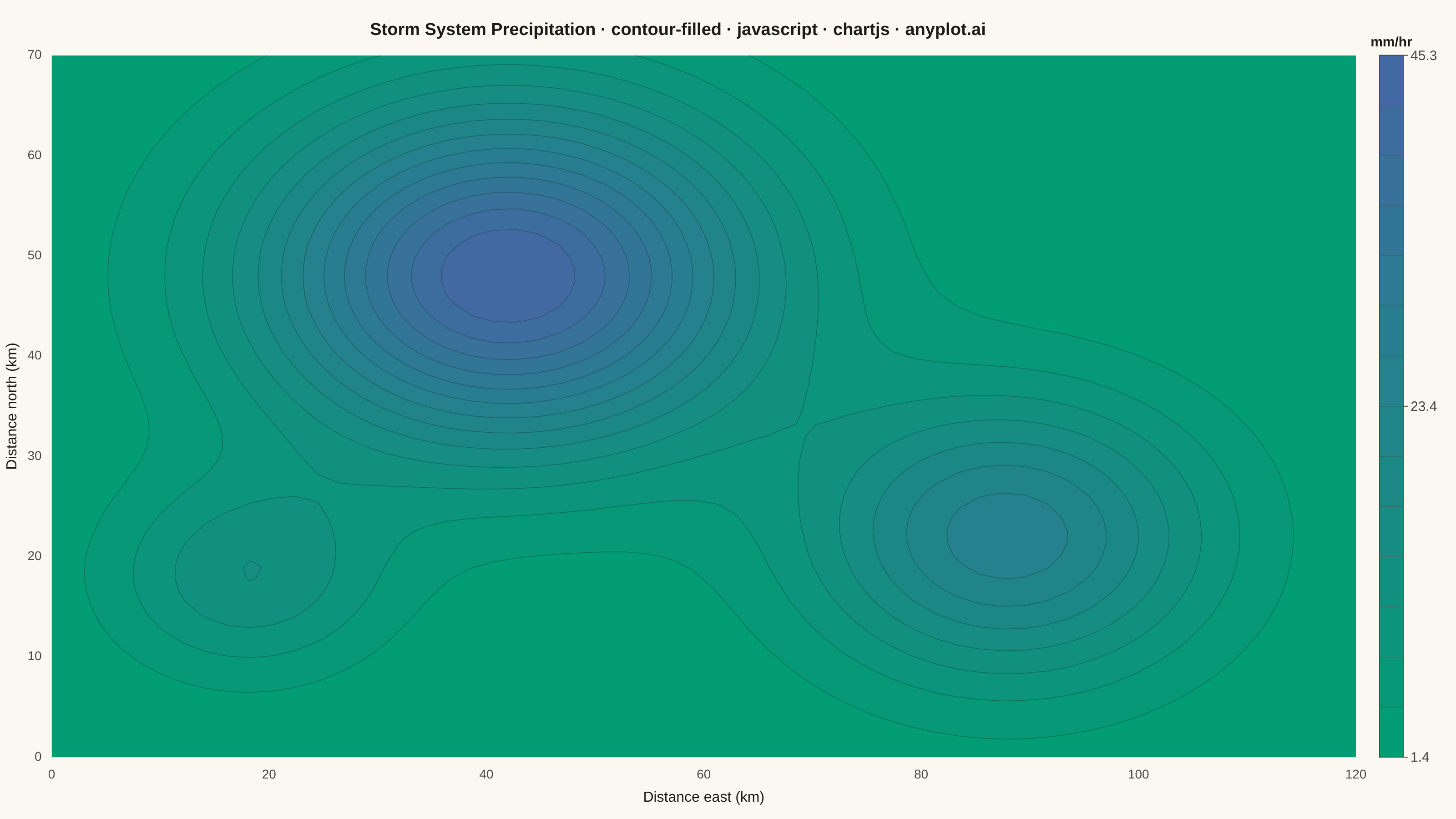
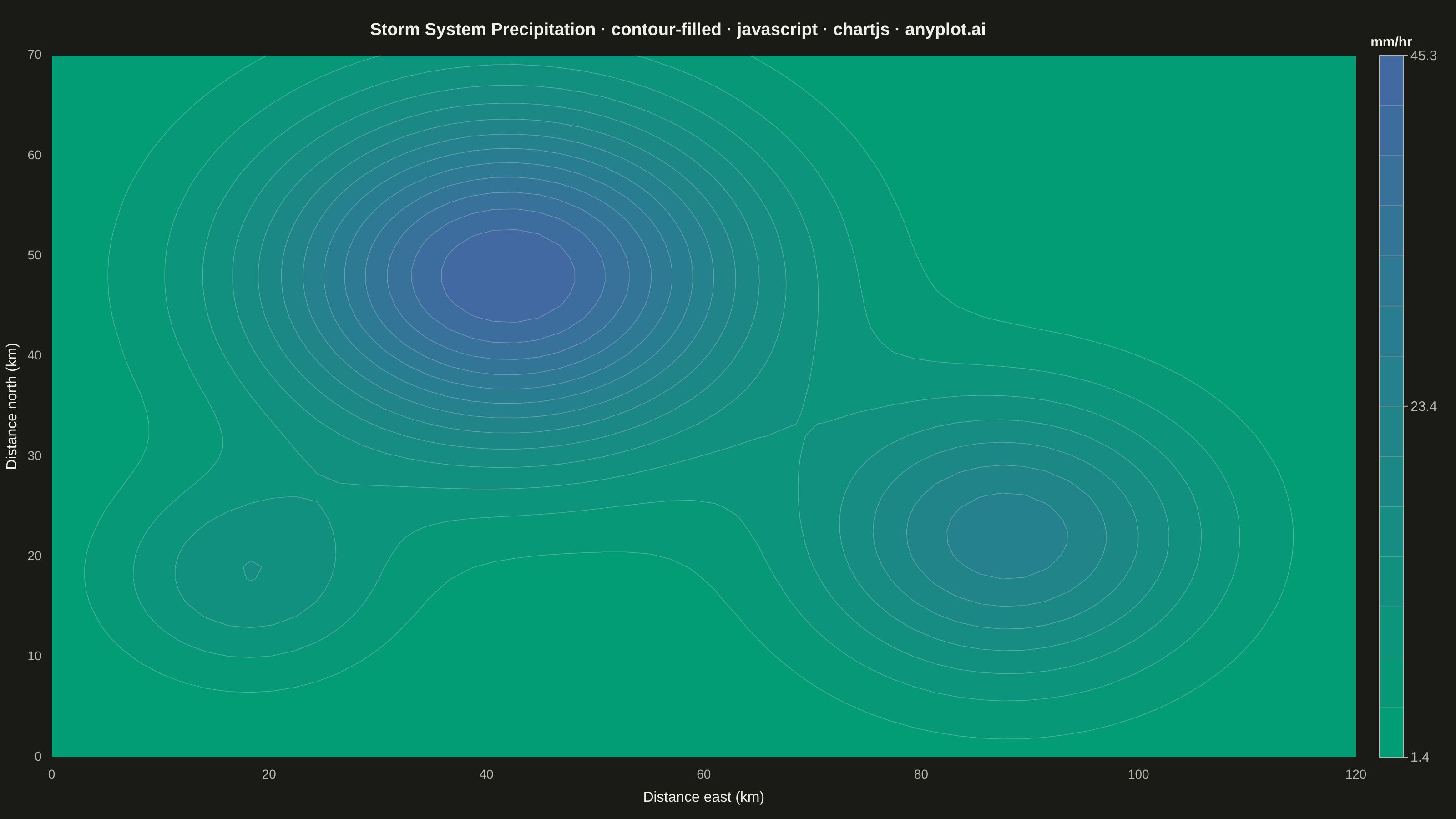
The same plot in 14 other libraries — JavaScript: D3.js, Apache ECharts, Highcharts, MUI X Charts; Python: Altair, Bokeh, lets-plot, Matplotlib, Plotly, plotnine, Pygal, Seaborn; R: ggplot2; Julia: Makie.jl. Compare all 15 side by side: Filled Contour Plot in Python, R, Julia and JavaScript.
A filled contour plot displays colored regions between level curves of a 2D scalar field, creating a smooth gradient visualization of continuous data. Unlike basic contour plots that show only isolines, filled contours use color bands to represent value ranges, making it easier to perceive gradual changes and identify regions of similar magnitude. This visualization is particularly effective for showing how a quantity varies continuously across a 2D surface.
// anyplot.ai
// contour-filled: Filled Contour Plot
// Library: chartjs 4.4.7 | JavaScript 22.23.2
// Quality: 94/100 | Created: 2026-09-04

//# anyplot-orientation: landscape

const t = window.ANYPLOT_TOKENS;

// --- Data: precipitation-intensity field over a regional grid --------------
// Chart.js has no native contour/isoband chart type (that lives in unpinned
// community plugins, out of scope). Instead this samples the field on a
// regular grid — exactly what the spec calls for — then rasterizes bilinearly
// interpolated, level-quantized bands via Chart.js's own draw-hook `plugins`
// API (native, not a plugin package) onto a real linear x/y coordinate system.
const N = 60;
const X_MIN = 0, X_MAX = 120; // km east
const Y_MIN = 0, Y_MAX = 70; // km north
const NUM_LEVELS = 14;

const xArr = [];
for (let i = 0; i < N; i++) xArr.push(X_MIN + ((X_MAX - X_MIN) * i) / (N - 1));
const yArr = [];
for (let j = 0; j < N; j++) yArr.push(Y_MIN + ((Y_MAX - Y_MIN) * j) / (N - 1));

function gaussianBump(x, y, cx, cy, sx, sy, amp) {
  const dx = (x - cx) / sx;
  const dy = (y - cy) / sy;
  return amp * Math.exp(-0.5 * (dx * dx + dy * dy));
}

// Three storm cells of different size/intensity over ambient drizzle — mm/hr,
// always >= 0 — for a more textured field than a symmetric two-bump pair.
let Z_MIN = Infinity, Z_MAX = -Infinity;
const zGrid = [];
for (let i = 0; i < N; i++) {
  zGrid.push([]);
  for (let j = 0; j < N; j++) {
    const x = xArr[i], y = yArr[j];
    const z =
      1.4 +
      gaussianBump(x, y, 42, 48, 16, 12, 44) +
      gaussianBump(x, y, 88, 22, 13, 10, 24) +
      gaussianBump(x, y, 18, 18, 9, 7, 12);
    zGrid[i].push(z);
    if (z < Z_MIN) Z_MIN = z;
    if (z > Z_MAX) Z_MAX = z;
  }
}
const LEVEL_STEP = (Z_MAX - Z_MIN) / NUM_LEVELS;

// --- Bilinear interpolation over the sampled grid ---------------------------
function gridFraction(v, vMin, vMax, count) {
  const f = ((v - vMin) / (vMax - vMin)) * (count - 1);
  const i0 = Math.max(0, Math.min(count - 2, Math.floor(f)));
  return { i0, frac: f - i0 };
}

function interpZ(x, y) {
  const gx = gridFraction(x, X_MIN, X_MAX, N);
  const gy = gridFraction(y, Y_MIN, Y_MAX, N);
  const z00 = zGrid[gx.i0][gy.i0];
  const z10 = zGrid[gx.i0 + 1][gy.i0];
  const z01 = zGrid[gx.i0][gy.i0 + 1];
  const z11 = zGrid[gx.i0 + 1][gy.i0 + 1];
  const zTop = z00 + (z10 - z00) * gx.frac;
  const zBot = z01 + (z11 - z01) * gx.frac;
  return zTop + (zBot - zTop) * gy.frac;
}

// --- Imprint sequential colormap (t.seq), quantized into level bands -------
function hexToRgb(hex) {
  return [parseInt(hex.slice(1, 3), 16), parseInt(hex.slice(3, 5), 16), parseInt(hex.slice(5, 7), 16)];
}
const SEQ_LO = hexToRgb(t.seq[0]);
const SEQ_HI = hexToRgb(t.seq[1]);

function levelOf(z) {
  let level = Math.floor((z - Z_MIN) / LEVEL_STEP);
  if (level >= NUM_LEVELS) level = NUM_LEVELS - 1;
  if (level < 0) level = 0;
  return level;
}

function bandRgb(level) {
  const frac = (level + 0.5) / NUM_LEVELS;
  return [
    Math.round(SEQ_LO[0] + (SEQ_HI[0] - SEQ_LO[0]) * frac),
    Math.round(SEQ_LO[1] + (SEQ_HI[1] - SEQ_LO[1]) * frac),
    Math.round(SEQ_LO[2] + (SEQ_HI[2] - SEQ_LO[2]) * frac),
  ];
}

// Renders the level-banded field into an offscreen raster canvas at a fixed
// pixel budget, then it gets scaled into the chart area by the draw plugin.
function renderBands(gridW, gridH) {
  const canvas = document.createElement("canvas");
  canvas.width = gridW;
  canvas.height = gridH;
  const ctx = canvas.getContext("2d");
  const img = ctx.createImageData(gridW, gridH);
  const data = img.data;
  for (let py = 0; py < gridH; py++) {
    const y = Y_MAX - (py / (gridH - 1)) * (Y_MAX - Y_MIN);
    for (let px = 0; px < gridW; px++) {
      const x = X_MIN + (px / (gridW - 1)) * (X_MAX - X_MIN);
      const [r, g, b] = bandRgb(levelOf(interpZ(x, y)));
      const idx = (py * gridW + px) * 4;
      data[idx] = r;
      data[idx + 1] = g;
      data[idx + 2] = b;
      data[idx + 3] = 255;
    }
  }
  ctx.putImageData(img, 0, 0);
  return canvas;
}

// --- Marching squares for the band-boundary isolines ------------------------
// For each 4-bit corner code (BL=bit0, BR=bit1, TR=bit2, TL=bit3, 1=above
// threshold), which pairs of edge indices connect as a line segment.
// Edges: 0=bottom (BL-BR), 1=right (BR-TR), 2=top (TL-TR), 3=left (BL-TL)
const SEG = [
  [], [[0, 3]], [[0, 1]], [[3, 1]],
  [[1, 2]], [[0, 3], [1, 2]], [[0, 2]], [[3, 2]],
  [[3, 2]], [[0, 2]], [[0, 1], [2, 3]], [[1, 2]],
  [[3, 1]], [[0, 1]], [[0, 3]], [],
];

// Precise levels for identification — every band boundary drawn as a thin
// isoline lets a viewer read off exact contour crossings within a band.
const isoThresholds = [];
for (let lvl = 1; lvl < NUM_LEVELS; lvl++) isoThresholds.push(Z_MIN + lvl * LEVEL_STEP);

// --- Mount -------------------------------------------------------------------
const canvas = document.createElement("canvas");
document.getElementById("container").appendChild(canvas);

let bandCanvas = null;

const contourPlugin = {
  id: "contourFill",
  afterDraw(chart) {
    const ctx = chart.ctx;
    const ca = chart.chartArea;
    if (!ca || !bandCanvas) return;
    const areaW = ca.right - ca.left;
    const areaH = ca.bottom - ca.top;

    ctx.save();
    ctx.drawImage(bandCanvas, ca.left, ca.top, areaW, areaH);

    // --- Isolines at every band boundary, clipped to the plot area ---------
    const xs = chart.scales.x, ys = chart.scales.y;
    const xPx = xArr.map((v) => xs.getPixelForValue(v));
    const yPx = yArr.map((v) => ys.getPixelForValue(v));

    function edgePx(e, i, j, z00, z10, z11, z01, thresh) {
      const f = (a, b, za, zb) => a + ((thresh - za) / (zb - za)) * (b - a);
      switch (e) {
        case 0: return [f(xPx[i], xPx[i + 1], z00, z10), yPx[j]];
        case 1: return [xPx[i + 1], f(yPx[j], yPx[j + 1], z10, z11)];
        case 2: return [f(xPx[i], xPx[i + 1], z01, z11), yPx[j + 1]];
        case 3: return [xPx[i], f(yPx[j], yPx[j + 1], z00, z01)];
      }
    }

    ctx.beginPath();
    ctx.rect(ca.left, ca.top, areaW, areaH);
    ctx.clip();
    ctx.beginPath();
    ctx.strokeStyle = t.ink;
    ctx.lineWidth = 0.75;
    ctx.globalAlpha = 0.3;
    for (const thresh of isoThresholds) {
      for (let i = 0; i < N - 1; i++) {
        for (let j = 0; j < N - 1; j++) {
          const z00 = zGrid[i][j], z10 = zGrid[i + 1][j];
          const z11 = zGrid[i + 1][j + 1], z01 = zGrid[i][j + 1];
          const code =
            (z00 >= thresh ? 1 : 0) | (z10 >= thresh ? 2 : 0) |
            (z11 >= thresh ? 4 : 0) | (z01 >= thresh ? 8 : 0);
          for (const [e0, e1] of SEG[code]) {
            const [ax, ay] = edgePx(e0, i, j, z00, z10, z11, z01, thresh);
            const [bx, by] = edgePx(e1, i, j, z00, z10, z11, z01, thresh);
            ctx.moveTo(ax, ay);
            ctx.lineTo(bx, by);
          }
        }
      }
    }
    ctx.stroke();
    ctx.restore();

    // --- Colorbar ------------------------------------------------------------
    const barX = ca.right + 26;
    const barW = 26;
    const barH = areaH;

    // Stepped bands matching the plot's own level quantization, so the
    // colorbar reads as the same 14 discrete bands rather than a smooth ramp.
    for (let level = 0; level < NUM_LEVELS; level++) {
      const [r, g, b] = bandRgb(level);
      const bandTop = ca.bottom - ((level + 1) / NUM_LEVELS) * barH;
      const bandHeight = barH / NUM_LEVELS;
      ctx.fillStyle = `rgb(${r}, ${g}, ${b})`;
      ctx.fillRect(barX, bandTop, barW, bandHeight);
    }
    ctx.strokeStyle = t.inkSoft;
    ctx.lineWidth = 0.75;
    ctx.globalAlpha = 0.5;
    for (let level = 1; level < NUM_LEVELS; level++) {
      const boundaryY = ca.bottom - (level / NUM_LEVELS) * barH;
      ctx.beginPath();
      ctx.moveTo(barX, boundaryY);
      ctx.lineTo(barX + barW, boundaryY);
      ctx.stroke();
    }
    ctx.globalAlpha = 1;
    ctx.lineWidth = 1;
    ctx.strokeRect(barX, ca.top, barW, barH);

    ctx.fillStyle = t.ink;
    ctx.font = "bold 15px sans-serif";
    ctx.textAlign = "center";
    ctx.fillText("mm/hr", barX + barW / 2, ca.top - 10);

    ctx.strokeStyle = t.inkSoft;
    ctx.fillStyle = t.inkSoft;
    ctx.font = "15px sans-serif";
    ctx.textAlign = "left";
    const ticks = [
      { frac: 1, label: Z_MAX.toFixed(1) },
      { frac: 0.5, label: ((Z_MIN + Z_MAX) / 2).toFixed(1) },
      { frac: 0, label: Z_MIN.toFixed(1) },
    ];
    for (const tk of ticks) {
      const ty = ca.bottom - tk.frac * barH;
      ctx.beginPath();
      ctx.moveTo(barX + barW, ty);
      ctx.lineTo(barX + barW + 5, ty);
      ctx.stroke();
      ctx.fillText(tk.label, barX + barW + 8, ty + 5);
    }
    ctx.restore();
  },
};

// --- Title (fontsize scales down when the title runs past the ~67-char
// mandated-title baseline — see prompts/plot-generator.md) ------------------
const TITLE = "Storm System Precipitation · contour-filled · javascript · chartjs · anyplot.ai";
const TITLE_DEFAULT_SIZE = 22;
const TITLE_FLOOR = 15;
const titleFontSize = Math.max(TITLE_FLOOR, Math.round(TITLE_DEFAULT_SIZE * Math.min(1, 67 / TITLE.length)));

// --- Chart -------------------------------------------------------------------
// A scatter chart with an empty dataset supplies the real linear x/y
// coordinate system the contourFill plugin draws the raster and isolines into.
const chart = new Chart(canvas, {
  type: "scatter",
  data: { datasets: [{ data: [] }] },
  options: {
    responsive: true,
    maintainAspectRatio: false,
    animation: false,
    layout: { padding: { right: 110, top: 10, bottom: 10 } },
    plugins: {
      title: {
        display: true,
        text: TITLE,
        color: t.ink,
        font: { size: titleFontSize },
        padding: { top: 12, bottom: 16 },
      },
      legend: { display: false },
    },
    scales: {
      x: {
        type: "linear",
        min: X_MIN,
        max: X_MAX,
        ticks: { color: t.inkSoft, font: { size: 14 } },
        grid: { display: false },
        title: { display: true, text: "Distance east (km)", color: t.ink, font: { size: 16 } },
      },
      y: {
        type: "linear",
        min: Y_MIN,
        max: Y_MAX,
        ticks: { color: t.inkSoft, font: { size: 14 } },
        grid: { display: false },
        title: { display: true, text: "Distance north (km)", color: t.ink, font: { size: 16 } },
      },
    },
  },
  plugins: [contourPlugin],
});

// Build the raster at a resolution matched to the chart area's aspect ratio,
// now that layout has settled and chartArea is known.
const area = chart.chartArea;
const areaAspect = (area.right - area.left) / (area.bottom - area.top);
const PIXEL_BUDGET = 520000;
const gridH = Math.round(Math.sqrt(PIXEL_BUDGET / areaAspect));
const gridW = Math.round(gridH * areaAspect);
bandCanvas = renderBands(gridW, gridH);

chart.update("none");

window.__anyplotReady = true;
Runnable source as JSON, for any HTTP client: https://api.anyplot.ai/specs/contour-filled/chartjs/code. Any spec id and library id listed in llms-full.txt fit the same URL shape; every URL below is complete and callable.
{
  "spec_id": "contour-filled",
  "language": "javascript",
  "library": "chartjs",
  "page": "https://anyplot.ai/contour-filled/javascript/chartjs",
  "hub": "https://anyplot.ai/contour-filled",
  "code_json": "https://api.anyplot.ai/specs/contour-filled/chartjs/code",
  "spec_json": "https://api.anyplot.ai/specs/contour-filled",
  "render_light_png": "https://storage.googleapis.com/anyplot-images/plots/contour-filled/javascript/chartjs/plot-light.png",
  "render_dark_png": "https://storage.googleapis.com/anyplot-images/plots/contour-filled/javascript/chartjs/plot-dark.png",
  "interactive_light_html": "https://storage.googleapis.com/anyplot-images/plots/contour-filled/javascript/chartjs/plot-light.html",
  "interactive_dark_html": "https://storage.googleapis.com/anyplot-images/plots/contour-filled/javascript/chartjs/plot-dark.html",
  "quality_score": 94.0,
  "license": "MIT",
  "guide": "https://anyplot.ai/llms.txt"
}
Part of Filled Contour Plot on anyplot.ai.