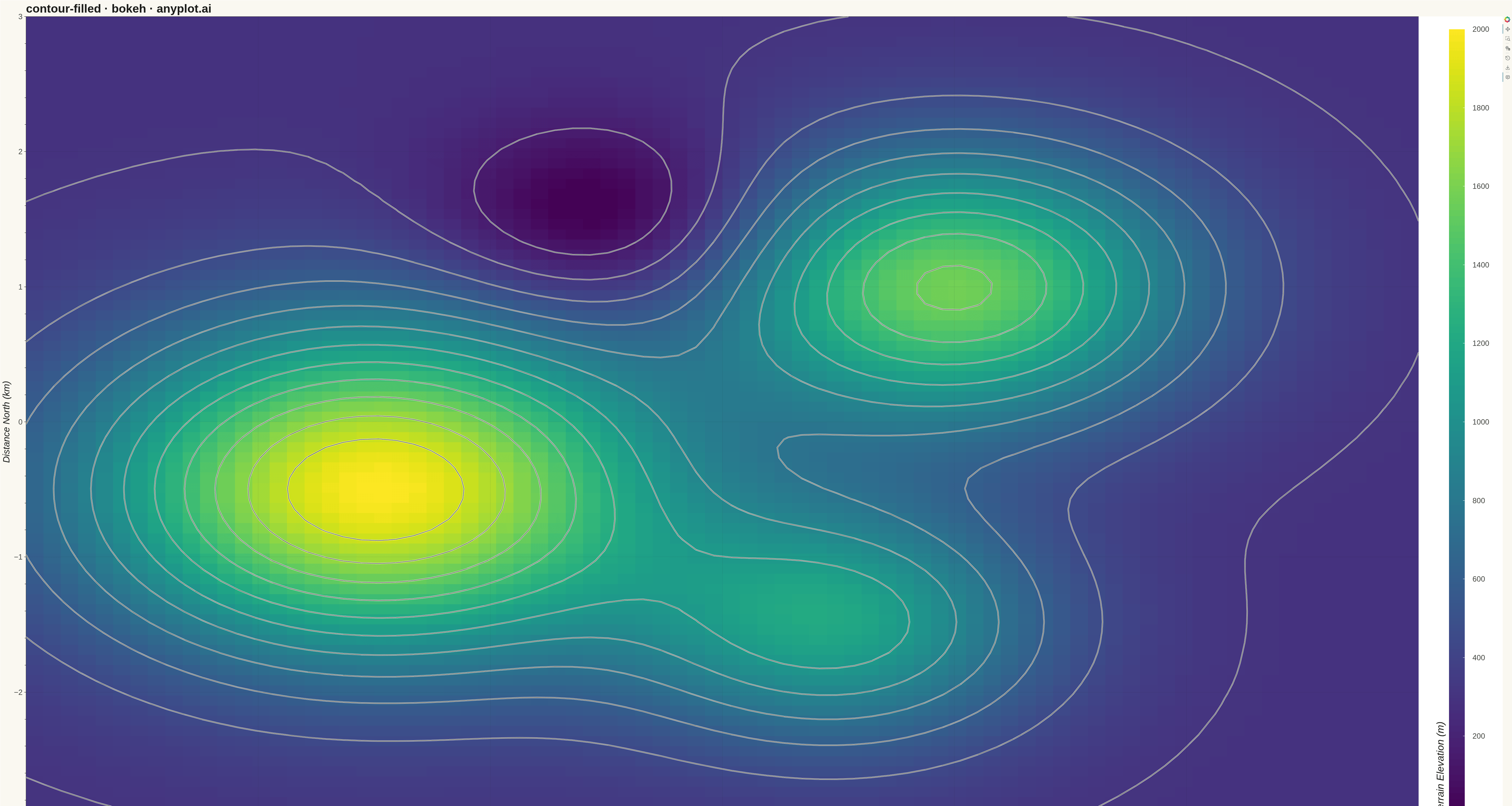
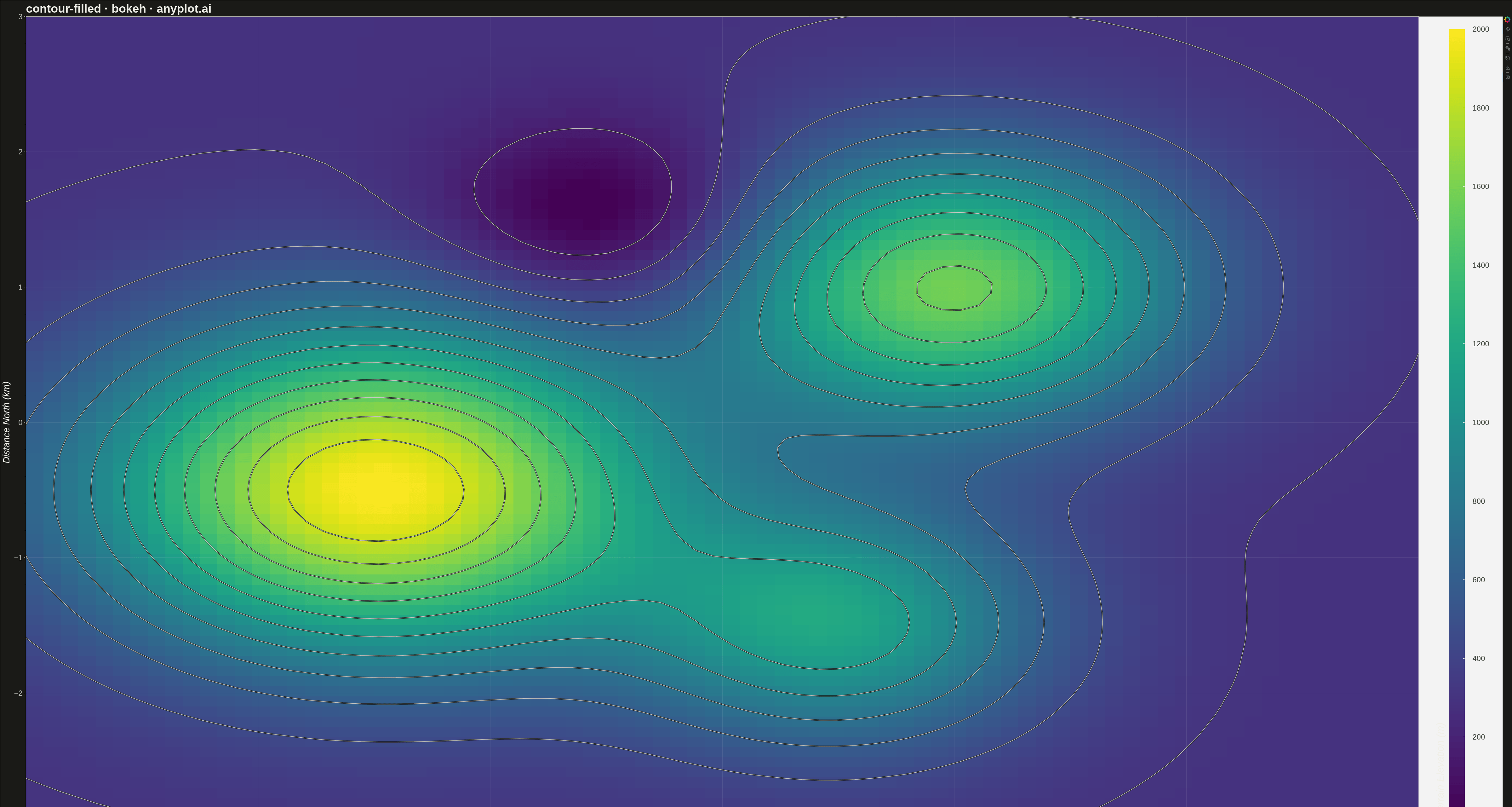
A filled contour plot displays colored regions between level curves of a 2D scalar field, creating a smooth gradient visualization of continuous data. Unlike basic contour plots that show only isolines, filled contours use color bands to represent value ranges, making it easier to perceive gradual changes and identify regions of similar magnitude. This visualization is particularly effective for showing how a quantity varies continuously across a 2D surface.
""" anyplot.ai
contour-filled: Filled Contour Plot
Library: bokeh 3.9.0 | Python 3.13.13
Quality: 86/100 | Updated: 2026-05-11
"""

import os
import time
from pathlib import Path

import bokeh.io
import bokeh.models
import bokeh.palettes
import bokeh.plotting
import numpy as np
from contourpy import contour_generator
from selenium import webdriver
from selenium.webdriver.chrome.options import Options


output_file = bokeh.io.output_file
save = bokeh.io.save
BasicTicker = bokeh.models.BasicTicker
ColorBar = bokeh.models.ColorBar
HoverTool = bokeh.models.HoverTool
LinearColorMapper = bokeh.models.LinearColorMapper
Viridis256 = bokeh.palettes.Viridis256
figure = bokeh.plotting.figure

# Theme tokens
THEME = os.getenv("ANYPLOT_THEME", "light")
PAGE_BG = "#FAF8F1" if THEME == "light" else "#1A1A17"
ELEVATED_BG = "#FFFDF6" if THEME == "light" else "#242420"
INK = "#1A1A17" if THEME == "light" else "#F0EFE8"
INK_SOFT = "#4A4A44" if THEME == "light" else "#B8B7B0"

# Data - Terrain elevation surface with multiple peaks
np.random.seed(42)
x = np.linspace(-3, 3, 80)
y = np.linspace(-3, 3, 80)
X, Y = np.meshgrid(x, y)

# Create surface with multiple Gaussian peaks (terrain elevation in meters)
Z = (
    1.5 * np.exp(-((X - 1) ** 2 + (Y - 1) ** 2))
    + 2.0 * np.exp(-((X + 1.5) ** 2 + (Y + 0.5) ** 2) / 1.5)
    + 1.0 * np.exp(-((X - 0.5) ** 2 + (Y + 1.5) ** 2) / 0.8)
    - 0.5 * np.exp(-((X + 0.5) ** 2 + (Y - 1.5) ** 2) / 0.5)
)

# Scale to realistic elevation values (0-2000 meters)
Z = (Z - Z.min()) / (Z.max() - Z.min()) * 2000

# Create figure at 4800x2700 px with interactive tools
p = figure(
    width=4800,
    height=2700,
    title="contour-filled · bokeh · anyplot.ai",
    x_range=(x.min(), x.max()),
    y_range=(y.min(), y.max()),
    tools="pan,wheel_zoom,box_zoom,reset,save",
)

# Explicitly set axis labels after figure creation
p.xaxis.axis_label = "Distance East (km)"
p.yaxis.axis_label = "Distance North (km)"

# Color mapper for the filled surface
color_mapper = LinearColorMapper(palette=Viridis256, low=Z.min(), high=Z.max())

# Draw the filled surface using image
p.image(image=[Z], x=x.min(), y=y.min(), dw=x.max() - x.min(), dh=y.max() - y.min(), color_mapper=color_mapper)

# Overlay contour lines at specific levels for precise identification
n_contour_lines = 12
contour_levels = np.linspace(Z.min(), Z.max(), n_contour_lines + 2)[1:-1]

# Create contour generator
cont_gen = contour_generator(x=X, y=Y, z=Z)

# Theme-aware contour line colors
contour_base = "#FFFDF6" if THEME == "light" else "#242420"
contour_outline = INK

# Draw contour lines with high contrast (base color + outline)
for level in contour_levels:
    lines = cont_gen.lines(level)
    for line in lines:
        # Draw base line for visibility
        p.line(line[:, 0], line[:, 1], line_width=4, color=contour_base, alpha=0.9)
        # Draw thinner outline on top for contrast
        p.line(line[:, 0], line[:, 1], line_width=1.5, color=contour_outline, alpha=0.8)

# Add colorbar with terrain context
color_bar = ColorBar(
    color_mapper=color_mapper,
    ticker=BasicTicker(desired_num_ticks=10),
    label_standoff=25,
    title="Terrain Elevation (m)",
    title_text_font_size="24pt",
    title_standoff=20,
    major_label_text_font_size="18pt",
    width=50,
    padding=40,
)
p.add_layout(color_bar, "right")

# Style text for large canvas
p.title.text_font_size = "28pt"
p.xaxis.axis_label_text_font_size = "22pt"
p.yaxis.axis_label_text_font_size = "22pt"
p.xaxis.major_label_text_font_size = "18pt"
p.yaxis.major_label_text_font_size = "18pt"

# Grid styling - very subtle with reduced opacity and width
p.xgrid.grid_line_color = INK
p.ygrid.grid_line_color = INK
p.xgrid.grid_line_alpha = 0.10
p.ygrid.grid_line_alpha = 0.10
p.xgrid.grid_line_width = 1
p.ygrid.grid_line_width = 1
p.xgrid.level = "overlay"
p.ygrid.level = "overlay"

# Add hover tool for interactive elevation display
# Create a grid of hover points for better interactivity
hover_x, hover_y, hover_z = [], [], []
step = 4  # Sample every 4th point for responsive hovering
for i in range(0, len(x), step):
    for j in range(0, len(y), step):
        hover_x.append(x[i])
        hover_y.append(y[j])
        hover_z.append(round(Z[j, i], 1))

# Add invisible scatter points for hover detection
hover_renderer = p.scatter(hover_x, hover_y, size=30, fill_alpha=0, line_alpha=0, name="hover_points")
hover_renderer.data_source.data["elevation"] = hover_z

# Configure hover tool to show elevation values
hover = HoverTool(
    renderers=[hover_renderer],
    tooltips=[("Location", "(@x{0.0} km E, @y{0.0} km N)"), ("Elevation", "@elevation{0} m")],
    mode="mouse",
)
p.add_tools(hover)

# Theme-adaptive chrome
p.background_fill_color = PAGE_BG
p.border_fill_color = PAGE_BG
p.outline_line_color = INK_SOFT

p.title.text_color = INK
p.xaxis.axis_label_text_color = INK
p.yaxis.axis_label_text_color = INK
p.xaxis.major_label_text_color = INK_SOFT
p.yaxis.major_label_text_color = INK_SOFT
p.xaxis.axis_line_color = INK_SOFT
p.yaxis.axis_line_color = INK_SOFT
p.xaxis.major_tick_line_color = INK_SOFT
p.yaxis.major_tick_line_color = INK_SOFT

if p.legend:
    p.legend.background_fill_color = ELEVATED_BG
    p.legend.border_line_color = INK_SOFT
    p.legend.label_text_color = INK_SOFT

# Colorbar text styling
if p.right:
    for renderer in p.right:
        if hasattr(renderer, "label_text_color"):
            renderer.label_text_color = INK_SOFT
        if hasattr(renderer, "title_text_color"):
            renderer.title_text_color = INK

# Save as HTML
output_file(f"plot-{THEME}.html")
save(p)

# Screenshot with Selenium
W, H = 4800, 2700
opts = Options()
for arg in (
    "--headless=new",
    "--no-sandbox",
    "--disable-dev-shm-usage",
    "--disable-gpu",
    f"--window-size={W},{H}",
    "--hide-scrollbars",
):
    opts.add_argument(arg)
driver = webdriver.Chrome(options=opts)
driver.set_window_size(W, H)
driver.get(f"file://{Path(f'plot-{THEME}.html').resolve()}")
time.sleep(3)
driver.save_screenshot(f"plot-{THEME}.png")
driver.quit()
Runnable source as JSON, for any HTTP client: https://api.anyplot.ai/specs/contour-filled/bokeh/code. Any spec id and library id listed in llms-full.txt fit the same URL shape; every URL below is complete and callable.
{
  "spec_id": "contour-filled",
  "language": "python",
  "library": "bokeh",
  "page": "https://anyplot.ai/contour-filled/python/bokeh",
  "hub": "https://anyplot.ai/contour-filled",
  "code_json": "https://api.anyplot.ai/specs/contour-filled/bokeh/code",
  "spec_json": "https://api.anyplot.ai/specs/contour-filled",
  "render_light_png": "https://storage.googleapis.com/anyplot-images/plots/contour-filled/python/bokeh/plot-light.png",
  "render_dark_png": "https://storage.googleapis.com/anyplot-images/plots/contour-filled/python/bokeh/plot-dark.png",
  "interactive_light_html": "https://storage.googleapis.com/anyplot-images/plots/contour-filled/python/bokeh/plot-light.html",
  "interactive_dark_html": "https://storage.googleapis.com/anyplot-images/plots/contour-filled/python/bokeh/plot-dark.html",
  "quality_score": 86.0,
  "license": "MIT",
  "guide": "https://anyplot.ai/llms.txt"
}
Part of Filled Contour Plot on anyplot.ai.