The same plot in 14 other libraries — JavaScript: Chart.js, Apache ECharts, Highcharts, MUI X Charts; Python: Altair, Bokeh, lets-plot, Matplotlib, Plotly, plotnine, Pygal, Seaborn; R: ggplot2; Julia: Makie.jl. Compare all 15 side by side: Filled Contour Plot in Python, R, Julia and JavaScript.
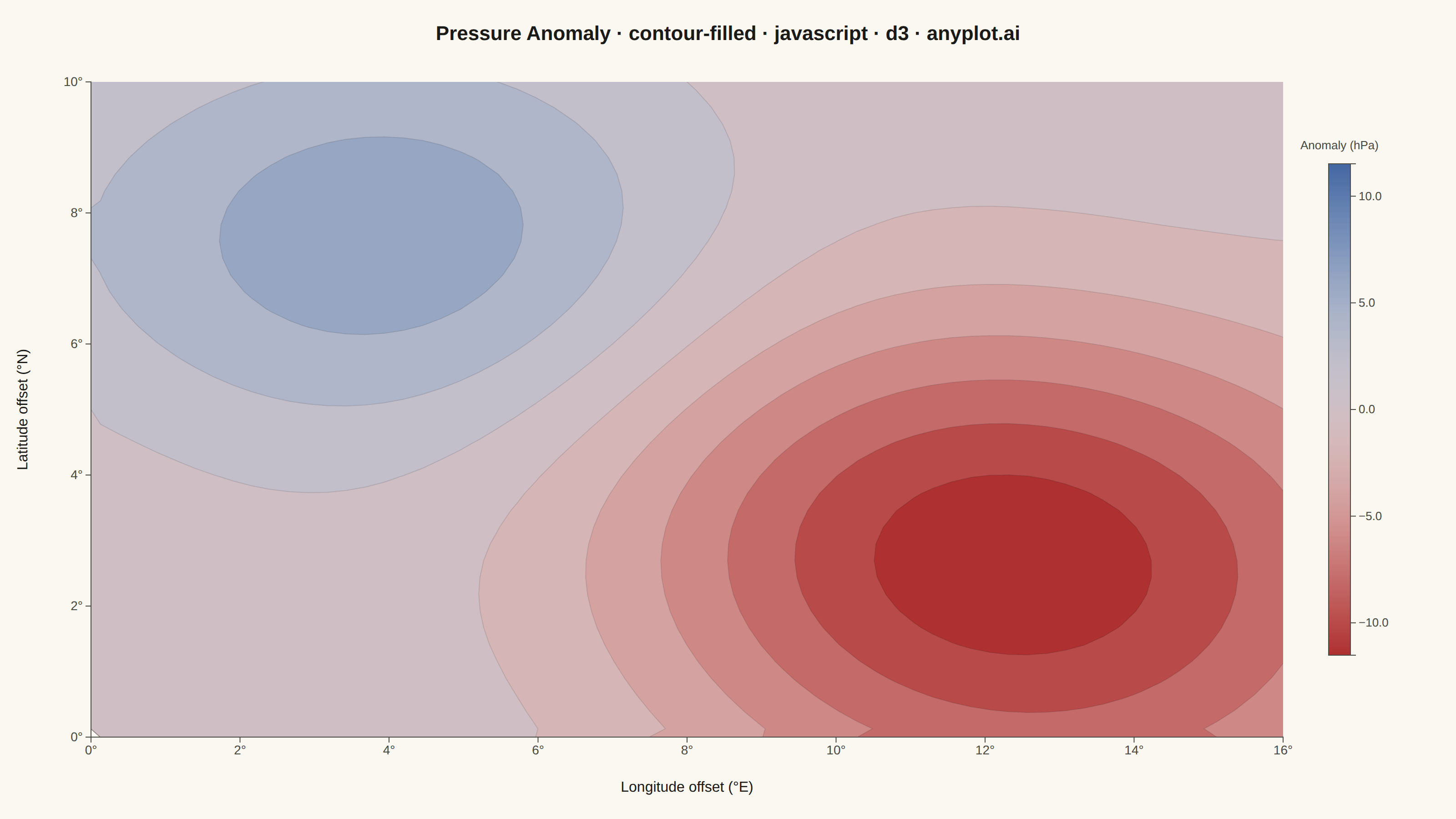
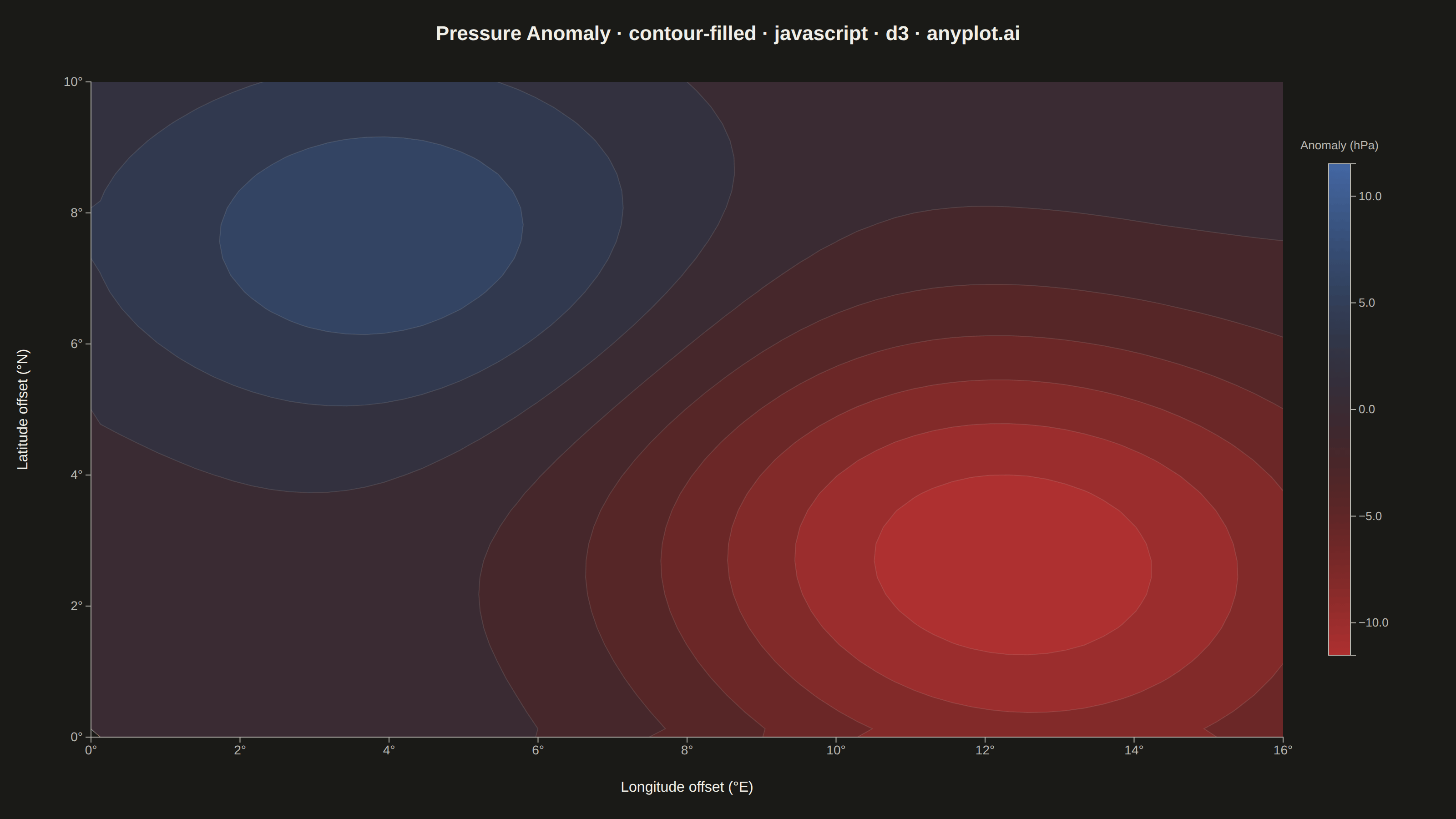
A filled contour plot displays colored regions between level curves of a 2D scalar field, creating a smooth gradient visualization of continuous data. Unlike basic contour plots that show only isolines, filled contours use color bands to represent value ranges, making it easier to perceive gradual changes and identify regions of similar magnitude. This visualization is particularly effective for showing how a quantity varies continuously across a 2D surface.
// anyplot.ai
// contour-filled: Filled Contour Plot
// Library: d3 7.9.0 | JavaScript 22.23.2
// Quality: 90/100 | Created: 2026-09-04

const t = window.ANYPLOT_TOKENS;
const { width: W, height: H } = window.ANYPLOT_SIZE;
const margin = { top: 90, right: 190, bottom: 90, left: 100 };
const iw = W - margin.left - margin.right;
const ih = H - margin.top - margin.bottom;

// --- Data: sea-level pressure anomaly on a regular lon/lat grid ------------
// Deterministic combination of a high-pressure ridge and a low-pressure
// trough plus a mild sinusoidal ripple, evaluated on a 64x40 mesh (within
// the spec's 30x30-100x100 range).
const gridWidth = 64;
const gridHeight = 40;
const lonMin = 0;
const lonMax = 16;
const latMin = 0;
const latMax = 10;

function pressureAnomaly(lon, lat) {
  const ridge = 9 * Math.exp(-(((lon - 4) ** 2) / (2 * 3.2 ** 2) + ((lat - 7.5) ** 2) / (2 * 2.4 ** 2)));
  const trough = -11 * Math.exp(-(((lon - 12) ** 2) / (2 * 3.6 ** 2) + ((lat - 2.8) ** 2) / (2 * 2.6 ** 2)));
  const ripple = 1.5 * Math.sin(lon / 3) * Math.cos(lat / 2.5);
  return ridge + trough + ripple;
}

const lonAt = (i) => lonMin + (i / (gridWidth - 1)) * (lonMax - lonMin);
const latAt = (j) => latMin + (j / (gridHeight - 1)) * (latMax - latMin);

const values = new Array(gridWidth * gridHeight);
for (let j = 0; j < gridHeight; j++) {
  for (let i = 0; i < gridWidth; i++) {
    values[j * gridWidth + i] = pressureAnomaly(lonAt(i), latAt(j));
  }
}
const [zMin, zMax] = d3.extent(values);
const maxAbs = Math.max(Math.abs(zMin), Math.abs(zMax));

// --- Scales ------------------------------------------------------------------
const lonScale = d3.scaleLinear().domain([lonMin, lonMax]).range([0, iw]);
const latScale = d3.scaleLinear().domain([latMin, latMax]).range([ih, 0]);
// Diverging colormap centered on the physically meaningful zero anomaly.
const colorScale = d3.scaleSequential(d3.interpolateRgbBasis(t.div)).domain([-maxAbs, maxAbs]);

// --- Contour bands (cumulative-area technique: each band is the full region
// >= its threshold, so painting low-to-high builds the filled color bands and
// each polygon boundary doubles as a precise isoline) --------------------------
const bands = d3.contours().size([gridWidth, gridHeight]).thresholds(14)(values);

const geoTransform = d3.geoTransform({
  point(px, py) {
    this.stream.point(lonScale(lonAt(px)), latScale(latAt(py)));
  },
});
const path = d3.geoPath(geoTransform);

// --- SVG mount ----------------------------------------------------------------
const svg = d3.select("#container").append("svg").attr("width", W).attr("height", H);
const g = svg.append("g").attr("transform", `translate(${margin.left},${margin.top})`);

// Clip so band polygons (which extend to the mesh border) never bleed past the plot area.
svg
  .append("clipPath")
  .attr("id", "plot-clip")
  .append("rect")
  .attr("width", iw)
  .attr("height", ih);

g.append("g")
  .attr("clip-path", "url(#plot-clip)")
  .selectAll("path")
  .data(bands)
  .join("path")
  .attr("d", path)
  .attr("fill", (d) => colorScale(d.value))
  .attr("stroke", t.ink)
  .attr("stroke-opacity", 0.12)
  .attr("stroke-width", 1);

// --- Axes ----------------------------------------------------------------------
const xAxis = g
  .append("g")
  .attr("transform", `translate(0,${ih})`)
  .call(d3.axisBottom(lonScale).ticks(8).tickFormat((d) => `${d}°`));
const yAxis = g.append("g").call(d3.axisLeft(latScale).ticks(6).tickFormat((d) => `${d}°`));
for (const axis of [xAxis, yAxis]) {
  axis.selectAll("text").attr("fill", t.inkSoft).style("font-size", "14px");
  axis.selectAll("line").attr("stroke", t.inkSoft);
  axis.select(".domain").attr("stroke", t.inkSoft);
}

g.append("text")
  .attr("x", iw / 2)
  .attr("y", ih + 60)
  .attr("text-anchor", "middle")
  .attr("fill", t.ink)
  .style("font-size", "16px")
  .text("Longitude offset (°E)");

g.append("text")
  .attr("transform", "rotate(-90)")
  .attr("x", -ih / 2)
  .attr("y", -70)
  .attr("text-anchor", "middle")
  .attr("fill", t.ink)
  .style("font-size", "16px")
  .text("Latitude offset (°N)");

// --- Colorbar legend ------------------------------------------------------------
const barX = iw + 50;
const barWidth = 24;
const barHeight = ih * 0.75;
const barY = (ih - barHeight) / 2;

const gradient = svg
  .append("defs")
  .append("linearGradient")
  .attr("id", "contour-legend-gradient")
  .attr("x1", "0%")
  .attr("x2", "0%")
  .attr("y1", "0%")
  .attr("y2", "100%");
const stopCount = 20;
for (let s = 0; s <= stopCount; s++) {
  const frac = s / stopCount;
  gradient
    .append("stop")
    .attr("offset", `${frac * 100}%`)
    .attr("stop-color", colorScale(maxAbs - frac * 2 * maxAbs));
}

const legend = g.append("g").attr("transform", `translate(${barX},0)`);
legend
  .append("rect")
  .attr("width", barWidth)
  .attr("height", barHeight)
  .attr("y", barY)
  .attr("fill", "url(#contour-legend-gradient)")
  .attr("stroke", t.inkSoft)
  .attr("stroke-width", 1);

const legendScale = d3.scaleLinear().domain([-maxAbs, maxAbs]).range([barY + barHeight, barY]);
const legendAxis = legend
  .append("g")
  .attr("transform", `translate(${barWidth},0)`)
  .call(d3.axisRight(legendScale).ticks(6).tickFormat(d3.format(".1f")));
legendAxis.selectAll("text").attr("fill", t.inkSoft).style("font-size", "13px");
legendAxis.selectAll("line").attr("stroke", t.inkSoft);
legendAxis.select(".domain").attr("stroke", t.inkSoft);

legend
  .append("text")
  .attr("x", barWidth / 2)
  .attr("y", barY - 16)
  .attr("text-anchor", "middle")
  .attr("fill", t.inkSoft)
  .style("font-size", "13px")
  .text("Anomaly (hPa)");

// --- Title ------------------------------------------------------------------
svg
  .append("text")
  .attr("x", W / 2)
  .attr("y", 44)
  .attr("text-anchor", "middle")
  .attr("fill", t.ink)
  .style("font-size", "22px")
  .style("font-weight", "600")
  .text("Pressure Anomaly · contour-filled · javascript · d3 · anyplot.ai");
Runnable source as JSON, for any HTTP client: https://api.anyplot.ai/specs/contour-filled/d3/code. Any spec id and library id listed in llms-full.txt fit the same URL shape; every URL below is complete and callable.
{
  "spec_id": "contour-filled",
  "language": "javascript",
  "library": "d3",
  "page": "https://anyplot.ai/contour-filled/javascript/d3",
  "hub": "https://anyplot.ai/contour-filled",
  "code_json": "https://api.anyplot.ai/specs/contour-filled/d3/code",
  "spec_json": "https://api.anyplot.ai/specs/contour-filled",
  "render_light_png": "https://storage.googleapis.com/anyplot-images/plots/contour-filled/javascript/d3/plot-light.png",
  "render_dark_png": "https://storage.googleapis.com/anyplot-images/plots/contour-filled/javascript/d3/plot-dark.png",
  "interactive_light_html": "https://storage.googleapis.com/anyplot-images/plots/contour-filled/javascript/d3/plot-light.html",
  "interactive_dark_html": "https://storage.googleapis.com/anyplot-images/plots/contour-filled/javascript/d3/plot-dark.html",
  "quality_score": 90.0,
  "license": "MIT",
  "guide": "https://anyplot.ai/llms.txt"
}
Part of Filled Contour Plot on anyplot.ai.