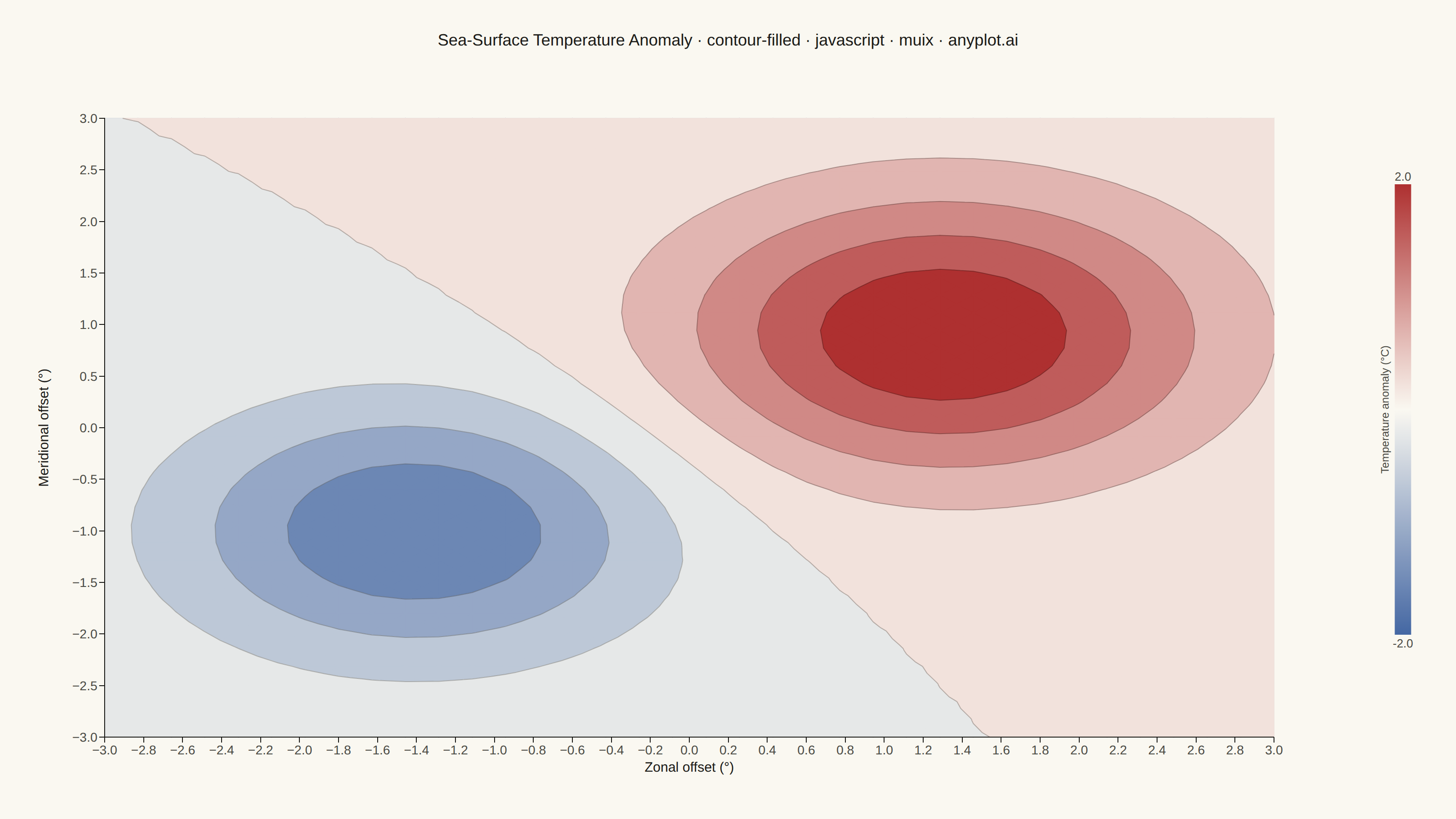
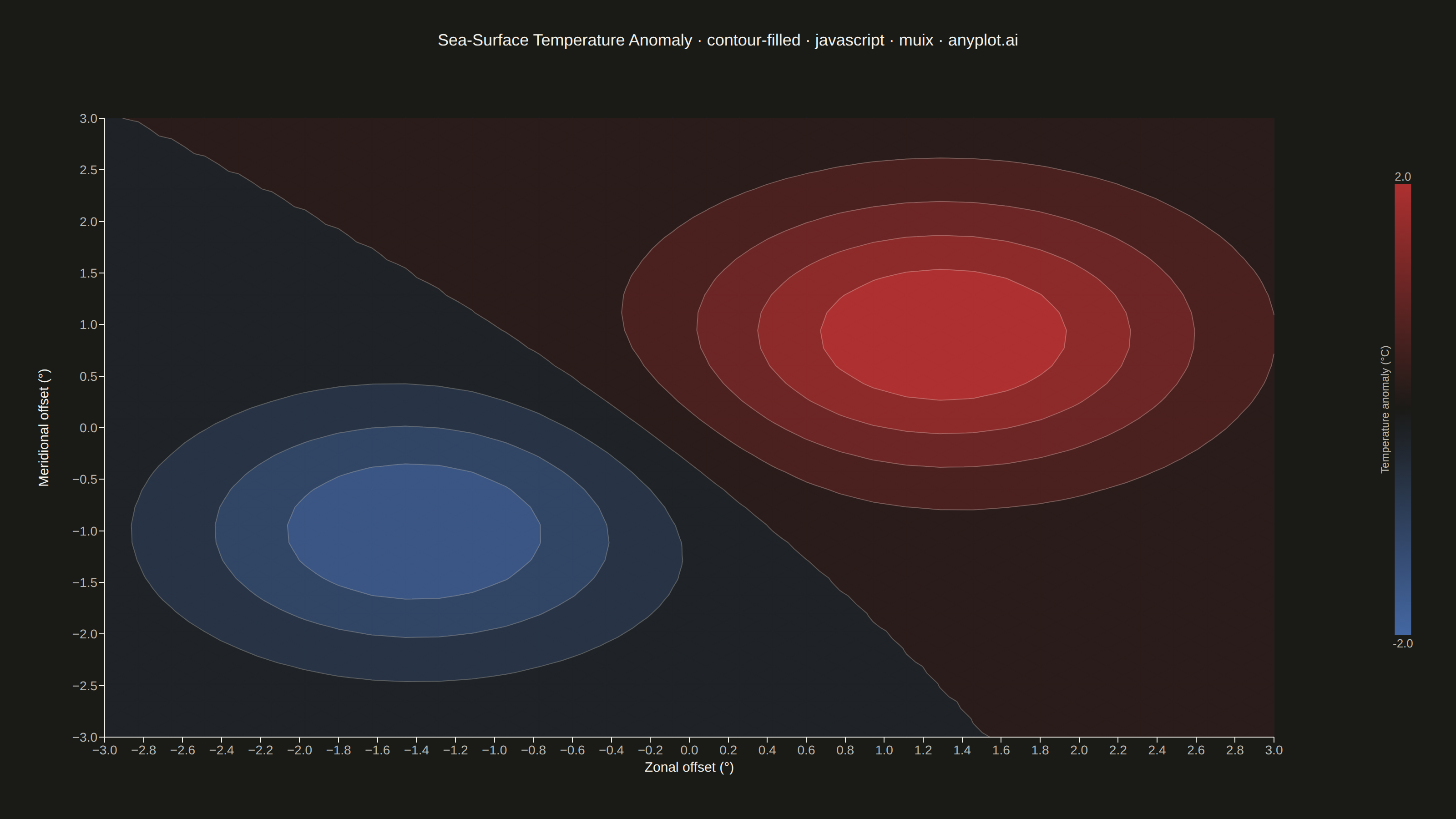
The same plot in 14 other libraries — JavaScript: Chart.js, D3.js, Apache ECharts, Highcharts; Python: Altair, Bokeh, lets-plot, Matplotlib, Plotly, plotnine, Pygal, Seaborn; R: ggplot2; Julia: Makie.jl. Compare all 15 side by side: Filled Contour Plot in Python, R, Julia and JavaScript.
A filled contour plot displays colored regions between level curves of a 2D scalar field, creating a smooth gradient visualization of continuous data. Unlike basic contour plots that show only isolines, filled contours use color bands to represent value ranges, making it easier to perceive gradual changes and identify regions of similar magnitude. This visualization is particularly effective for showing how a quantity varies continuously across a 2D surface.
// anyplot.ai
// contour-filled: Filled Contour Plot
// Library: muix 7.29.1 | JavaScript 22.23.2
// Quality: 84/100 | Updated: 2026-09-05
//# anyplot-orientation: landscape
// anyplot.ai
// contour-filled: Filled Contour Plot
// Library: MUI X Charts | React | Node 22
// License: @mui/x-charts — MIT (community). Pro/Premium are out of scope.
// Quality: pending | Created: 2026-09-04

import { ChartContainer } from "@mui/x-charts/ChartContainer";
import { ChartsXAxis } from "@mui/x-charts/ChartsXAxis";
import { ChartsYAxis } from "@mui/x-charts/ChartsYAxis";
import { ChartsText } from "@mui/x-charts/ChartsText";
import { ContinuousColorLegend } from "@mui/x-charts/ChartsLegend";
import { useXScale, useYScale } from "@mui/x-charts/hooks";

const t = window.ANYPLOT_TOKENS;
const SIZE = window.ANYPLOT_SIZE;

// --- Grid setup (in-memory, deterministic) ----------------------------------
const GRID = 36;
const X_MIN = -3, X_MAX = 3, Y_MIN = -3, Y_MAX = 3;

const xs = Array.from({ length: GRID }, (_, i) => X_MIN + (i / (GRID - 1)) * (X_MAX - X_MIN));
const ys = Array.from({ length: GRID }, (_, j) => Y_MIN + (j / (GRID - 1)) * (Y_MAX - Y_MIN));

// --- Scalar field: sea-surface temperature anomaly (warm patch + cool patch) ---
// Two Gaussian bumps only — kept free of high-frequency terms so the grid
// resolution below fully resolves every extremum (no sub-cell artifacts).
function anomaly(x, y) {
  const warmPatch = 2.0 * Math.exp(-((x - 1.3) * (x - 1.3) + (y - 0.9) * (y - 0.9)) * 0.55);
  const coolPatch = -1.6 * Math.exp(-((x + 1.4) * (x + 1.4) + (y + 1.0) * (y + 1.0)) * 0.65);
  return warmPatch + coolPatch;
}

// zGrid[j][i] = z at (xs[i], ys[j])
const zGrid = ys.map((y) => xs.map((x) => anomaly(x, y)));
const allZ = zGrid.flat();
const zMin = Math.min(...allZ);
const zMax = Math.max(...allZ);
const vAbs = Math.max(Math.abs(zMin), Math.abs(zMax));

// --- Imprint diverging colormap: t.div = [red, midpoint, blue] -------------
function hexToRgb(hex) {
  const int = parseInt(hex.slice(1), 16);
  return [(int >> 16) & 255, (int >> 8) & 255, int & 255];
}

function lerpChannel(a, b, ratio) {
  return Math.round(a + (b - a) * ratio);
}

function imprintDivInterpolator(stops) {
  const [low, mid, high] = stops.map(hexToRgb);
  return (position) => {
    const [start, end, localRatio] =
      position < 0.5 ? [low, mid, position / 0.5] : [mid, high, (position - 0.5) / 0.5];
    const [r, g, b] = [0, 1, 2].map((channel) =>
      lerpChannel(start[channel], end[channel], localRatio),
    );
    return `rgb(${r}, ${g}, ${b})`;
  };
}

// Reversed so position 0 (coolest/lowest z) lands on the blue end and
// position 1 (warmest/highest z) lands on the red end -- matching the
// universal warm=red / cool=blue temperature-anomaly convention.
const divColor = imprintDivInterpolator([...t.div].reverse());

// --- Band levels: symmetric around zero so the midpoint band sits at anomaly=0 ---
const NUM_BANDS = 10;
const levels = Array.from({ length: NUM_BANDS }, (_, k) => -vAbs + (k * 2 * vAbs) / NUM_BANDS);
const bandColors = Array.from({ length: NUM_BANDS }, (_, k) => divColor(k / (NUM_BANDS - 1)));

// --- Marching-triangles filled-contour geometry -----------------------------
// Each grid cell is split into 4 triangles around its centroid so every
// super-level-set boundary resolves without the marching-squares saddle
// ambiguity. Super-level sets are always nested (threshold_hi >= threshold_lo
// implies region_hi ⊆ region_lo), so painting bands low-to-high with a
// standard painter's algorithm produces correct filled contour bands
// regardless of how many disjoint blobs the field has.
function buildTriangles() {
  const tris = [];
  for (let j = 0; j < GRID - 1; j += 1) {
    for (let i = 0; i < GRID - 1; i += 1) {
      const sw = { x: xs[i], y: ys[j], z: zGrid[j][i] };
      const se = { x: xs[i + 1], y: ys[j], z: zGrid[j][i + 1] };
      const ne = { x: xs[i + 1], y: ys[j + 1], z: zGrid[j + 1][i + 1] };
      const nw = { x: xs[i], y: ys[j + 1], z: zGrid[j + 1][i] };
      const center = {
        x: (sw.x + se.x) / 2,
        y: (sw.y + nw.y) / 2,
        z: (sw.z + se.z + ne.z + nw.z) / 4,
      };
      tris.push([sw, se, center], [se, ne, center], [ne, nw, center], [nw, sw, center]);
    }
  }
  return tris;
}

const triangles = buildTriangles();

// Filled sub-polygon(s) of one triangle lying at/above `threshold`, plus the
// interpolated edge (if any) that traces the exact level curve through it.
function triangleFill(a, b, c, threshold) {
  const inA = a.z >= threshold, inB = b.z >= threshold, inC = c.z >= threshold;
  const nIn = (inA ? 1 : 0) + (inB ? 1 : 0) + (inC ? 1 : 0);
  const cross = (p, q) => {
    const ratio = (threshold - p.z) / (q.z - p.z);
    return { x: p.x + ratio * (q.x - p.x), y: p.y + ratio * (q.y - p.y) };
  };

  if (nIn === 0) return { polys: [], cut: null };
  if (nIn === 3) return { polys: [[a, b, c]], cut: null };

  if (nIn === 1) {
    if (inA) { const ab = cross(a, b), ca = cross(c, a); return { polys: [[a, ab, ca]], cut: [ab, ca] }; }
    if (inB) { const ab = cross(a, b), bc = cross(b, c); return { polys: [[b, bc, ab]], cut: [bc, ab] }; }
    const ca = cross(c, a), bc = cross(b, c);
    return { polys: [[c, ca, bc]], cut: [ca, bc] };
  }

  // nIn === 2 (exactly one vertex out)
  if (!inC) { const bc = cross(b, c), ca = cross(c, a); return { polys: [[a, b, bc, ca]], cut: [ca, bc] }; }
  if (!inA) { const ca = cross(c, a), ab = cross(a, b); return { polys: [[b, c, ca, ab]], cut: [ab, ca] }; }
  const ab = cross(a, b), bc = cross(b, c);
  return { polys: [[c, a, ab, bc]], cut: [bc, ab] };
}

// Bands k=1..NUM_BANDS-1 are computed from the triangulation; band k=0 is the
// full domain rect (everything is above zMin), painted first as the base layer.
const bandGeometry = [];
const isolineGeometry = [];
for (let k = 1; k < NUM_BANDS; k += 1) {
  const threshold = levels[k];
  const polys = [];
  const segments = [];
  for (const tri of triangles) {
    const { polys: p, cut } = triangleFill(tri[0], tri[1], tri[2], threshold);
    if (p.length) polys.push(...p);
    if (cut) segments.push(cut);
  }
  bandGeometry.push(polys);
  isolineGeometry.push(segments);
}

// --- Custom SVG layer: filled bands + isolines, mapped through the chart's own scales ---
function FilledContourLayer() {
  const xScale = useXScale();
  const yScale = useYScale();
  const toSVG = (x, y) => [xScale(x), yScale(y)];

  const polysToPath = (polys) =>
    polys
      .map((poly) => {
        const pts = poly.map((p) => toSVG(p.x, p.y));
        const head = `M ${pts[0][0].toFixed(1)},${pts[0][1].toFixed(1)}`;
        const tail = pts.slice(1).map(([px, py]) => `L ${px.toFixed(1)},${py.toFixed(1)}`).join(" ");
        return `${head} ${tail} Z`;
      })
      .join(" ");

  const segmentsToPath = (segments) =>
    segments
      .map(([p0, p1]) => {
        const [x0, y0] = toSVG(p0.x, p0.y);
        const [x1, y1] = toSVG(p1.x, p1.y);
        return `M ${x0.toFixed(1)},${y0.toFixed(1)} L ${x1.toFixed(1)},${y1.toFixed(1)}`;
      })
      .join(" ");

  const [rx0, ry0] = toSVG(X_MIN, Y_MIN);
  const [rx1, ry1] = toSVG(X_MAX, Y_MAX);
  const baseRect = `M ${rx0.toFixed(1)},${ry0.toFixed(1)} L ${rx1.toFixed(1)},${ry0.toFixed(1)} L ${rx1.toFixed(1)},${ry1.toFixed(1)} L ${rx0.toFixed(1)},${ry1.toFixed(1)} Z`;

  return (
    <g>
      {/* Base band: fills the whole domain, subsequent bands paint over it (painter's algorithm) */}
      <path d={baseRect} fill={bandColors[0]} stroke={bandColors[0]} strokeWidth={0.75} />
      {bandGeometry.map((polys, idx) => (
        <path
          key={`band-${idx}`}
          d={polysToPath(polys)}
          fill={bandColors[idx + 1]}
          stroke={bandColors[idx + 1]}
          strokeWidth={0.75}
        />
      ))}
      {isolineGeometry.map((segments, idx) => (
        <path
          key={`iso-${idx}`}
          d={segmentsToPath(segments)}
          stroke={t.ink}
          strokeOpacity={0.28}
          strokeWidth={1}
          fill="none"
        />
      ))}
    </g>
  );
}

// --- Chart (default-exported component — the harness mounts it) -------------
const TITLE = "Sea-Surface Temperature Anomaly · contour-filled · javascript · muix · anyplot.ai";
const TITLE_FONT_SIZE = Math.max(15, Math.round(22 * Math.min(1, 67 / TITLE.length)));
const MARGIN = { top: 130, right: 200, bottom: 90, left: 115 };

// ContinuousColorLegend anchors flush against the literal SVG width, ignoring
// MARGIN.right entirely (its `position: "right"` offset is `svgWidth -
// legendWidth`, ie. the very last canvas column) -- so the whole right-side
// cluster (legend + its rotated axis title) is wrapped in this leftward shift
// to keep tick-label glyphs off the true edge.
const RIGHT_EDGE_INSET = 48;

export default function Chart() {
  return (
    <ChartContainer
      width={SIZE.width}
      height={SIZE.height}
      series={[]}
      margin={MARGIN}
      skipAnimation
      xAxis={[
        {
          scaleType: "linear",
          min: X_MIN,
          max: X_MAX,
          label: "Zonal offset (°)",
          labelStyle: { fontSize: 15, fill: t.ink },
          tickLabelStyle: { fontSize: 14, fill: t.inkSoft },
        },
      ]}
      yAxis={[
        {
          scaleType: "linear",
          min: Y_MIN,
          max: Y_MAX,
          label: "Meridional offset (°)",
          labelStyle: { fontSize: 15, fill: t.ink },
          tickLabelStyle: { fontSize: 14, fill: t.inkSoft },
          // Push the rotated axis label further from the axis line than the
          // library's default offset, which collides with wide tick digits
          // like "-3.0" -- see ChartsYAxis's labelRefPoint formula.
          slotProps: { axisLabel: { x: -62 } },
        },
      ]}
      zAxis={[
        {
          colorMap: {
            type: "continuous",
            min: -vAbs,
            max: vAbs,
            color: divColor,
          },
        },
      ]}
    >
      <FilledContourLayer />
      <ChartsXAxis />
      <ChartsYAxis />
      <g transform={`translate(${-RIGHT_EDGE_INSET}, 0)`}>
        <ContinuousColorLegend
          position={{ horizontal: "right", vertical: "middle" }}
          direction="column"
          length="55%"
          thickness={18}
          labelStyle={{ fontSize: 13, fill: t.inkSoft }}
          minLabel={({ value }) => value.toFixed(1)}
          maxLabel={({ value }) => value.toFixed(1)}
        />
        <ChartsText
          text="Temperature anomaly (°C)"
          x={SIZE.width - 26}
          y={SIZE.height / 2}
          style={{ fontSize: 12, fill: t.inkSoft, textAnchor: "middle", angle: -90 }}
        />
      </g>
      <ChartsText
        text={TITLE}
        x={SIZE.width / 2}
        y={50}
        style={{ fontSize: TITLE_FONT_SIZE, fontWeight: 500, fill: t.ink, textAnchor: "middle" }}
      />
    </ChartContainer>
  );
}
Runnable source as JSON, for any HTTP client: https://api.anyplot.ai/specs/contour-filled/muix/code. Any spec id and library id listed in llms-full.txt fit the same URL shape; every URL below is complete and callable.
{
  "spec_id": "contour-filled",
  "language": "javascript",
  "library": "muix",
  "page": "https://anyplot.ai/contour-filled/javascript/muix",
  "hub": "https://anyplot.ai/contour-filled",
  "code_json": "https://api.anyplot.ai/specs/contour-filled/muix/code",
  "spec_json": "https://api.anyplot.ai/specs/contour-filled",
  "render_light_png": "https://storage.googleapis.com/anyplot-images/plots/contour-filled/javascript/muix/plot-light.png",
  "render_dark_png": "https://storage.googleapis.com/anyplot-images/plots/contour-filled/javascript/muix/plot-dark.png",
  "interactive_light_html": "https://storage.googleapis.com/anyplot-images/plots/contour-filled/javascript/muix/plot-light.html",
  "interactive_dark_html": "https://storage.googleapis.com/anyplot-images/plots/contour-filled/javascript/muix/plot-dark.html",
  "quality_score": 84.0,
  "license": "MIT",
  "guide": "https://anyplot.ai/llms.txt"
}
Part of Filled Contour Plot on anyplot.ai.