The same plot in 14 other libraries — Python: Altair, Bokeh, lets-plot, Matplotlib, Plotly, plotnine, Pygal, Seaborn; R: ggplot2; JavaScript: Chart.js, D3.js, Apache ECharts, Highcharts, MUI X Charts. Compare all 15 side by side: Feynman Diagram for Particle Interactions in Python, R, Julia and JavaScript.
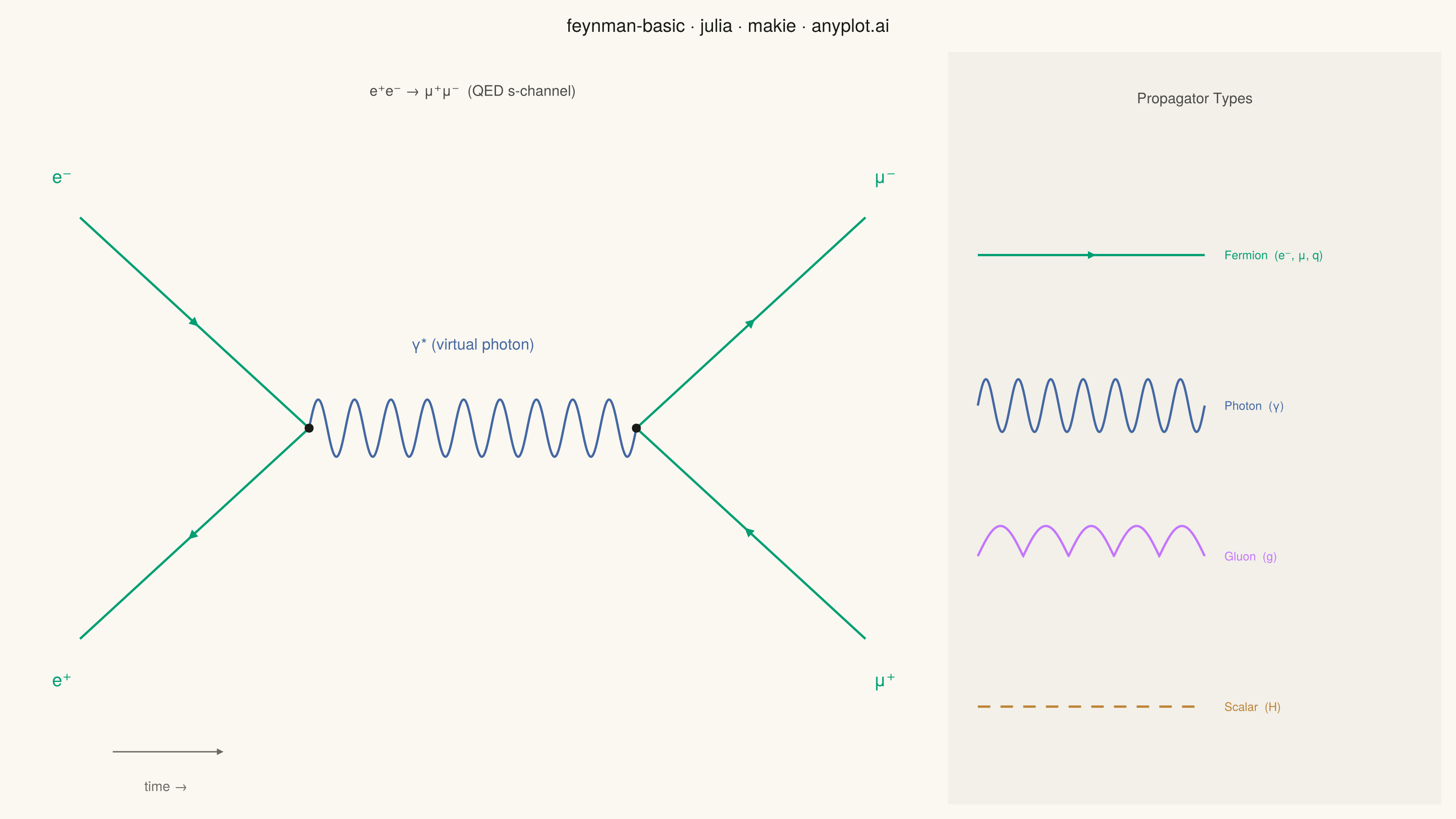
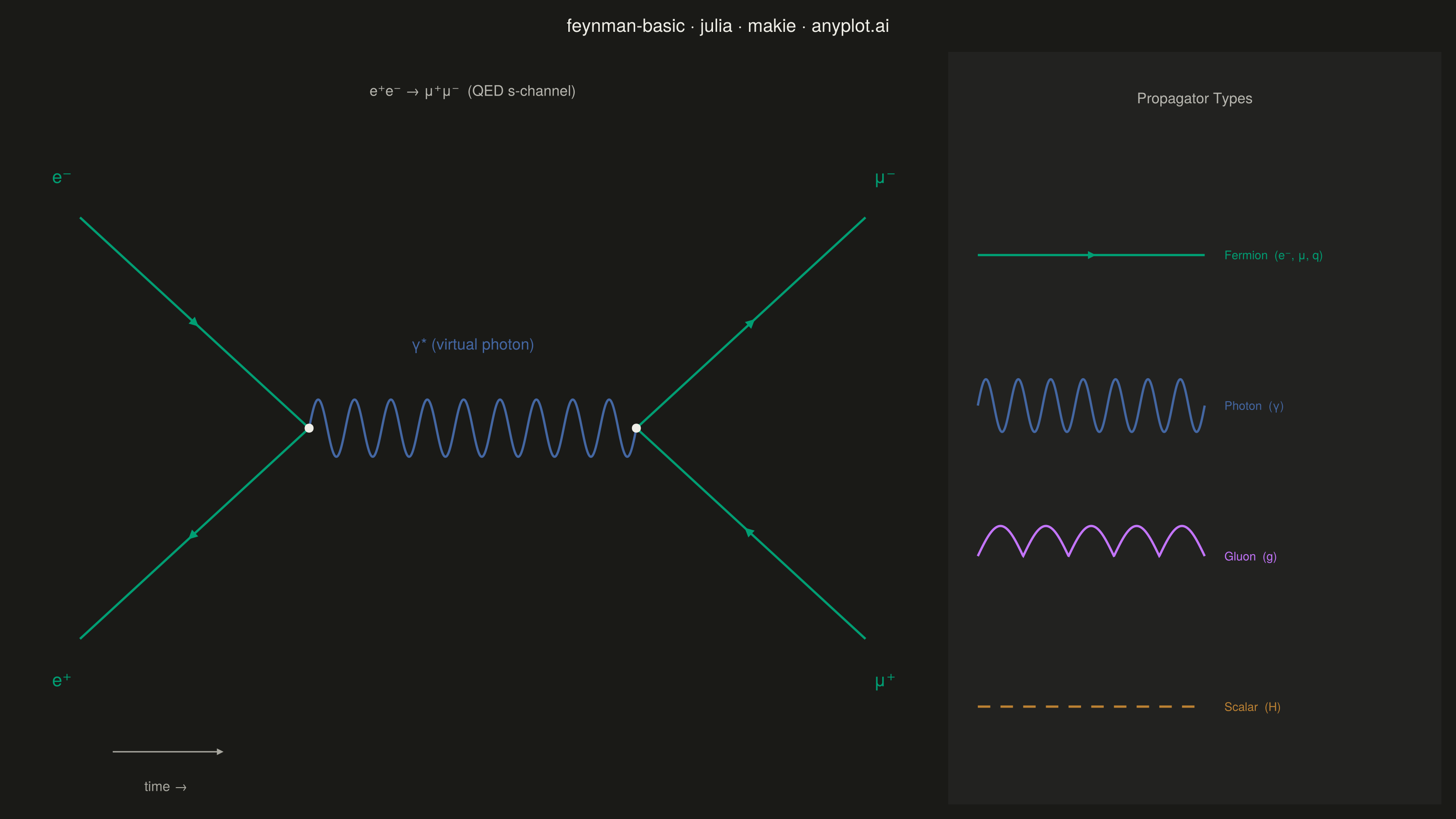
A Feynman diagram visualizes interactions between subatomic particles in quantum field theory. Different line styles represent different particle types: straight lines for fermions (electrons, quarks), wavy lines for photons, curly/looped lines for gluons, and dashed lines for scalar bosons (e.g., Higgs). Lines meet at vertices representing interaction points. Invented by Richard Feynman, these diagrams are both a computational tool and a cultural icon of modern physics.
# anyplot.ai
# feynman-basic: Feynman Diagram for Particle Interactions
# Library: makie 0.22.10 | Julia 1.11.9
# Quality: 93/100 | Created: 2026-06-03

using CairoMakie
using Colors
using Random

Random.seed!(42)

const THEME     = get(ENV, "ANYPLOT_THEME", "light")
const PAGE_BG   = THEME == "light" ? colorant"#FAF8F1" : colorant"#1A1A17"
const PANEL_BG  = THEME == "light" ? colorant"#F2F0E9" : colorant"#222220"
const INK       = THEME == "light" ? colorant"#1A1A17" : colorant"#F0EFE8"
const INK_SOFT  = THEME == "light" ? colorant"#4A4A44" : colorant"#B8B7B0"
const INK_MUTED = THEME == "light" ? colorant"#6B6A63" : colorant"#A8A79F"

const FERMION_COLOR = colorant"#009E73"  # brand green  (e-, e+, μ-, μ+, quarks)
const GLUON_COLOR   = colorant"#C475FD"  # lavender     (gluons / QCD)
const PHOTON_COLOR  = colorant"#4467A3"  # blue         (photons / EM bosons)
const SCALAR_COLOR  = colorant"#BD8233"  # ochre        (scalar bosons / Higgs)

# ─── Makie @recipe: composable Feynman propagator plot types ─────────────────
# Each recipe becomes a reusable, composable CairoMakie primitive — a Makie-
# exclusive feature that makes the diagram grammar extensible and domain-specific.

# Fermion propagator: solid line with a midpoint direction arrow
@recipe(FermionProp, xs, ys, direction) do scene
    Attributes(
        color     = FERMION_COLOR,
        linewidth = 2.5,
        arrowsize = 14,
    )
end

function Makie.plot!(fp::FermionProp)
    xs        = fp[1][]
    ys        = fp[2][]
    direction = fp[3][]   # 1 = particle (forward), -1 = antiparticle (backward)
    clr       = fp.color[]
    lw        = fp.linewidth[]
    arrsz     = fp.arrowsize[]

    lines!(fp, xs, ys; color = clr, linewidth = lw)

    n   = length(xs)
    mid = n ÷ 2
    dx  = xs[min(mid + 1, n)] - xs[max(mid - 1, 1)]
    dy  = ys[min(mid + 1, n)] - ys[max(mid - 1, 1)]
    len = sqrt(dx^2 + dy^2)
    if len > 1e-9
        arrows!(fp, [xs[mid]], [ys[mid]],
                [direction * 0.001 * dx / len],
                [direction * 0.001 * dy / len];
                arrowsize = arrsz, color = clr, linewidth = 0)
    end
    fp
end

# Photon propagator: transverse sinusoidal wave
@recipe(PhotonProp, x1, y1, x2, y2) do scene
    Attributes(
        color     = PHOTON_COLOR,
        linewidth = 2.5,
        n_waves   = 9,
        amplitude = 0.038,
    )
end

function Makie.plot!(pp::PhotonProp)
    x1, y1 = pp[1][], pp[2][]
    x2, y2 = pp[3][], pp[4][]
    clr     = pp.color[]
    lw      = pp.linewidth[]
    nw      = pp.n_waves[]
    amp     = pp.amplitude[]

    dx  = x2 - x1; dy = y2 - y1
    len = sqrt(dx^2 + dy^2)
    nx  = -dy / len; ny = dx / len   # unit normal (transverse direction)

    t    = LinRange(0.0, 1.0, 600)
    xs_w = @. x1 + t * dx + amp * sin(nw * 2π * t) * nx
    ys_w = @. y1 + t * dy + amp * sin(nw * 2π * t) * ny
    lines!(pp, xs_w, ys_w; color = clr, linewidth = lw)
    pp
end

# Gluon propagator: one-sided curly bumps via |sin| — visually distinct from photon
@recipe(GluonProp, x1, y1, x2, y2) do scene
    Attributes(
        color     = GLUON_COLOR,
        linewidth = 2.5,
        n_loops   = 7,
        amplitude = 0.048,
    )
end

function Makie.plot!(gp::GluonProp)
    x1, y1 = gp[1][], gp[2][]
    x2, y2 = gp[3][], gp[4][]
    clr     = gp.color[]
    lw      = gp.linewidth[]
    nl      = gp.n_loops[]
    amp     = gp.amplitude[]

    dx  = x2 - x1; dy = y2 - y1
    len = sqrt(dx^2 + dy^2)
    nx  = -dy / len; ny = dx / len

    t    = LinRange(0.0, 1.0, 800)
    xs_c = @. x1 + t * dx + amp * abs(sin(nl * π * t)) * nx
    ys_c = @. y1 + t * dy + amp * abs(sin(nl * π * t)) * ny
    lines!(gp, xs_c, ys_c; color = clr, linewidth = lw)
    gp
end

# Scalar boson propagator: dashed line (Higgs, etc.)
@recipe(ScalarProp, x1, y1, x2, y2) do scene
    Attributes(
        color     = SCALAR_COLOR,
        linewidth = 2.5,
        n_dashes  = 12,
    )
end

function Makie.plot!(sp::ScalarProp)
    x1, y1 = sp[1][], sp[2][]
    x2, y2 = sp[3][], sp[4][]
    clr     = sp.color[]
    lw      = sp.linewidth[]
    nd      = sp.n_dashes[]

    xs_d = Float64[]
    ys_d = Float64[]
    for i in 0:(nd - 1)
        t0 = i / nd
        t1 = (i + 0.55) / nd
        push!(xs_d, x1 + t0 * (x2 - x1), x1 + t1 * (x2 - x1), NaN)
        push!(ys_d, y1 + t0 * (y2 - y1), y1 + t1 * (y2 - y1), NaN)
    end
    lines!(sp, xs_d, ys_d; color = clr, linewidth = lw)
    sp
end

# ─── Figure: two-panel GridLayout ────────────────────────────────────────────
fig = Figure(
    size            = (1600, 900),
    fontsize        = 14,
    backgroundcolor = PAGE_BG,
)

# Title spans both columns
Label(fig[0, 1:2], "feynman-basic · julia · makie · anyplot.ai";
      fontsize = 20, color = INK, halign = :center)

# ─── Left panel: QED e+e- → μ+μ- s-channel diagram ──────────────────────────
ax = Axis(fig[1, 1];
    backgroundcolor    = PAGE_BG,
    topspinevisible    = false,
    rightspinevisible  = false,
    leftspinevisible   = false,
    bottomspinevisible = false,
    xgridvisible       = false,
    ygridvisible       = false,
    xticksvisible      = false,
    yticksvisible      = false,
    xticklabelsvisible = false,
    yticklabelsvisible = false,
)
xlims!(ax, -0.06, 1.06)
ylims!(ax, 0.0, 1.0)

text!(ax, 0.50, 0.96;
      text = "e⁺e⁻ → μ⁺μ⁻  (QED s-channel)",
      fontsize = 16, color = INK_SOFT, align = (:center, :top))

# Vertex positions
v1x, v1y = 0.30, 0.50
v2x, v2y = 0.70, 0.50

# External leg endpoints
em_x0, em_y0   = 0.02, 0.78   # e-  incoming top-left
ep_x0, ep_y0   = 0.02, 0.22   # e+  incoming bottom-left
mum_x1, mum_y1 = 0.98, 0.78   # μ-  outgoing top-right
mup_x1, mup_y1 = 0.98, 0.22   # μ+  outgoing bottom-right

n_pts = 100
fermionprop!(ax, LinRange(em_x0, v1x, n_pts), LinRange(em_y0, v1y, n_pts), 1)
fermionprop!(ax, LinRange(ep_x0, v1x, n_pts), LinRange(ep_y0, v1y, n_pts), -1)
fermionprop!(ax, LinRange(v2x, mum_x1, n_pts), LinRange(v2y, mum_y1, n_pts), 1)
fermionprop!(ax, LinRange(v2x, mup_x1, n_pts), LinRange(v2y, mup_y1, n_pts), -1)

photonprop!(ax, v1x, v1y, v2x, v2y)

scatter!(ax, [v1x, v2x], [v1y, v2y]; color = INK, markersize = 14, strokewidth = 0)

text!(ax, em_x0 - 0.01, em_y0 + 0.04;
      text = "e⁻", fontsize = 20, color = FERMION_COLOR, align = (:right, :bottom))
text!(ax, ep_x0 - 0.01, ep_y0 - 0.04;
      text = "e⁺", fontsize = 20, color = FERMION_COLOR, align = (:right, :top))
text!(ax, mum_x1 + 0.01, mum_y1 + 0.04;
      text = "μ⁻", fontsize = 20, color = FERMION_COLOR, align = (:left, :bottom))
text!(ax, mup_x1 + 0.01, mup_y1 - 0.04;
      text = "μ⁺", fontsize = 20, color = FERMION_COLOR, align = (:left, :top))
text!(ax, (v1x + v2x) / 2, v1y + 0.10;
      text = "γ* (virtual photon)", fontsize = 17, color = PHOTON_COLOR,
      align = (:center, :bottom))

arrows!(ax, [0.06], [0.07], [0.13], [0.0];
        arrowsize = 10, color = INK_MUTED, linewidth = 1.5)
text!(ax, 0.125, 0.035;
      text = "time →", fontsize = 15, color = INK_MUTED, align = (:center, :top))

# ─── Right panel: Propagator type reference ───────────────────────────────────
ax2 = Axis(fig[1, 2];
    backgroundcolor    = PANEL_BG,
    topspinevisible    = false,
    rightspinevisible  = false,
    leftspinevisible   = false,
    bottomspinevisible = false,
    xgridvisible       = false,
    ygridvisible       = false,
    xticksvisible      = false,
    yticksvisible      = false,
    xticklabelsvisible = false,
    yticklabelsvisible = false,
)
xlims!(ax2, 0.0, 1.0)
ylims!(ax2, 0.0, 1.0)

text!(ax2, 0.50, 0.95;
      text = "Propagator Types", fontsize = 16, color = INK_SOFT, align = (:center, :top))

prop_ys     = [0.73, 0.53, 0.33, 0.13]
prop_labels = ["Fermion  (e⁻, μ, q)", "Photon  (γ)", "Gluon  (g)", "Scalar  (H)"]
prop_colors = [FERMION_COLOR, PHOTON_COLOR, GLUON_COLOR, SCALAR_COLOR]

fermionprop!(ax2, LinRange(0.06, 0.52, n_pts), fill(prop_ys[1], n_pts), 1;
             color = FERMION_COLOR, arrowsize = 12)
photonprop!(ax2, 0.06, prop_ys[2], 0.52, prop_ys[2];
            color = PHOTON_COLOR, n_waves = 7, amplitude = 0.035)
gluonprop!(ax2, 0.06, prop_ys[3], 0.52, prop_ys[3];
           color = GLUON_COLOR, n_loops = 5, amplitude = 0.04)
scalarprop!(ax2, 0.06, prop_ys[4], 0.52, prop_ys[4];
            color = SCALAR_COLOR, n_dashes = 10)

for (y, lbl, clr) in zip(prop_ys, prop_labels, prop_colors)
    text!(ax2, 0.56, y; text = lbl, fontsize = 13, color = clr, align = (:left, :center))
end

# Column widths: 65% main diagram, 35% reference panel
colsize!(fig.layout, 1, Relative(0.65))
colsize!(fig.layout, 2, Relative(0.35))

save("plot-$(THEME).png", fig; px_per_unit = 2)
Runnable source as JSON, for any HTTP client: https://api.anyplot.ai/specs/feynman-basic/makie/code. Any spec id and library id listed in llms-full.txt fit the same URL shape; every URL below is complete and callable.
{
  "spec_id": "feynman-basic",
  "language": "julia",
  "library": "makie",
  "page": "https://anyplot.ai/feynman-basic/julia/makie",
  "hub": "https://anyplot.ai/feynman-basic",
  "code_json": "https://api.anyplot.ai/specs/feynman-basic/makie/code",
  "spec_json": "https://api.anyplot.ai/specs/feynman-basic",
  "render_light_png": "https://storage.googleapis.com/anyplot-images/plots/feynman-basic/julia/makie/plot-light.png",
  "render_dark_png": "https://storage.googleapis.com/anyplot-images/plots/feynman-basic/julia/makie/plot-dark.png",
  "quality_score": 93.0,
  "license": "MIT",
  "guide": "https://anyplot.ai/llms.txt"
}
Part of Feynman Diagram for Particle Interactions on anyplot.ai.