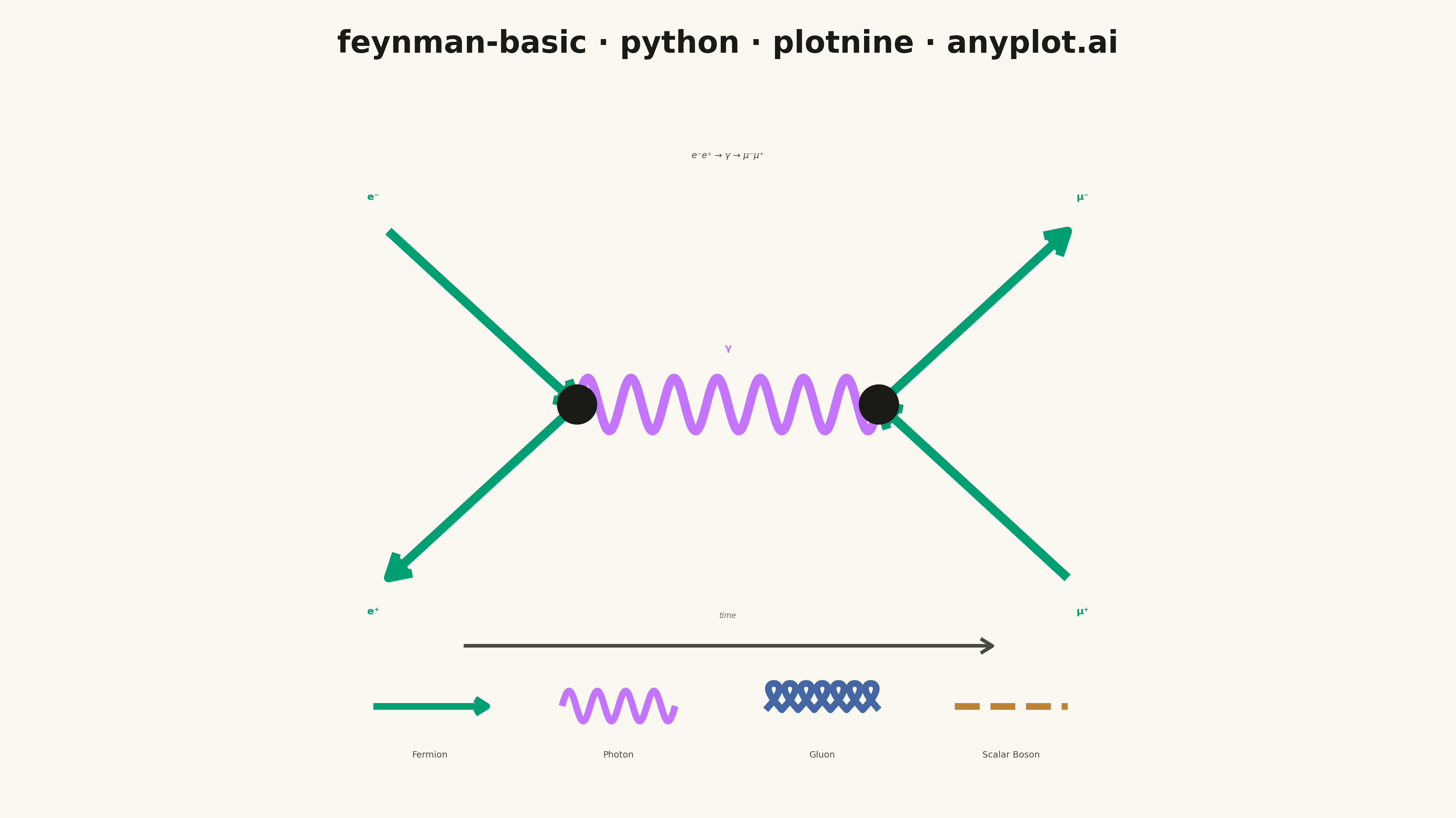
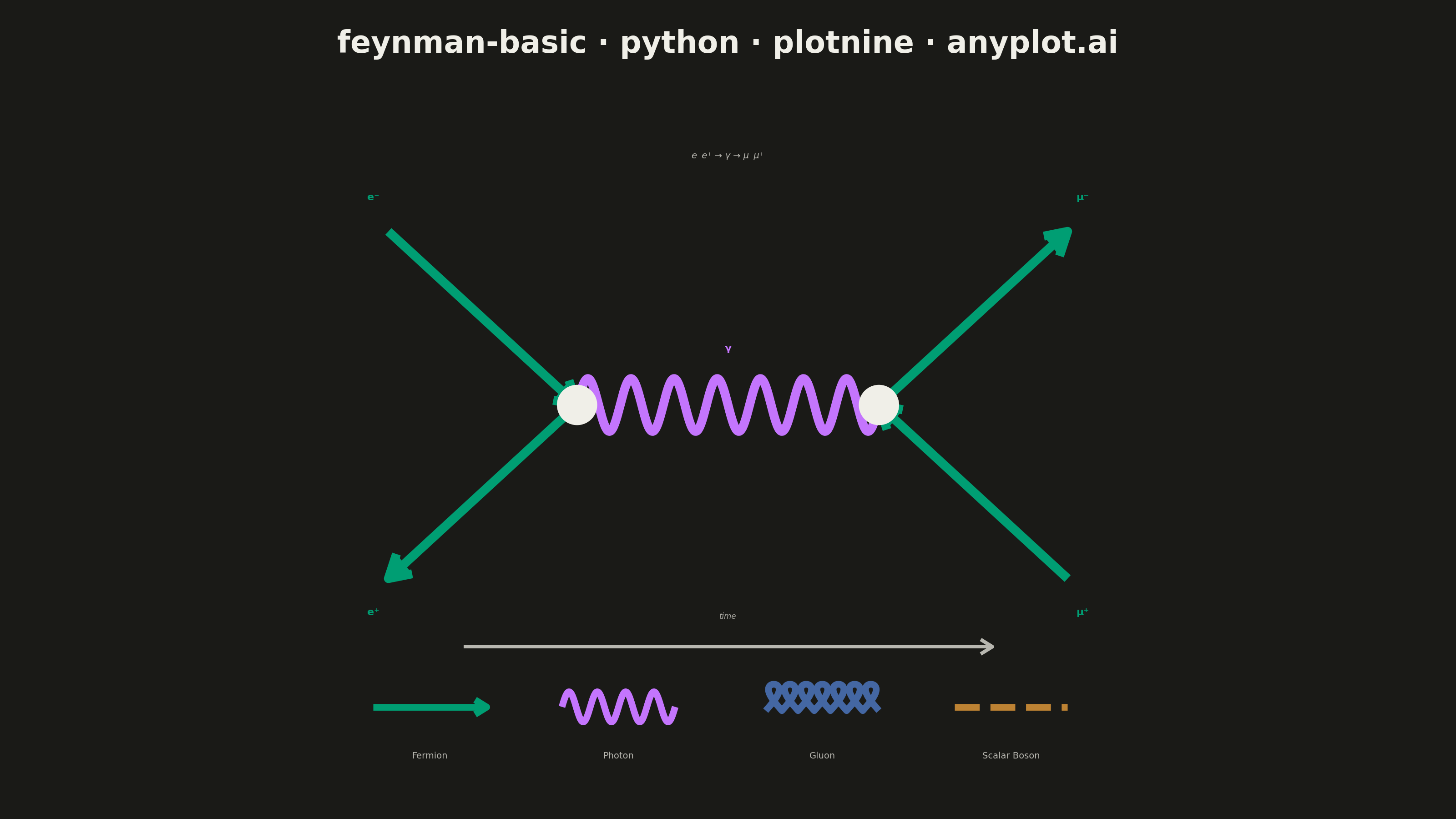
A Feynman diagram visualizes interactions between subatomic particles in quantum field theory. Different line styles represent different particle types: straight lines for fermions (electrons, quarks), wavy lines for photons, curly/looped lines for gluons, and dashed lines for scalar bosons (e.g., Higgs). Lines meet at vertices representing interaction points. Invented by Richard Feynman, these diagrams are both a computational tool and a cultural icon of modern physics.
""" anyplot.ai
feynman-basic: Feynman Diagram for Particle Interactions
Library: plotnine 0.15.5 | Python 3.13.13
Quality: 90/100 | Updated: 2026-06-03
"""

import os
import sys


# This file is named plotnine.py; remove its directory from sys.path so the
# installed plotnine package is found instead of this script.
_here = os.path.abspath(os.path.dirname(__file__))
sys.path = [p for p in sys.path if os.path.abspath(p or ".") != _here]
del _here

import numpy as np
import pandas as pd
from plotnine import (
    aes,
    annotate,
    arrow,
    coord_fixed,
    element_rect,
    element_text,
    geom_path,
    geom_point,
    geom_segment,
    geom_text,
    ggplot,
    labs,
    scale_color_manual,
    scale_x_continuous,
    scale_y_continuous,
    theme,
    theme_void,
)


# Theme-adaptive chrome tokens (Imprint palette, canonical)
THEME = os.getenv("ANYPLOT_THEME", "light")
PAGE_BG = "#FAF8F1" if THEME == "light" else "#1A1A17"
INK = "#1A1A17" if THEME == "light" else "#F0EFE8"
INK_SOFT = "#4A4A44" if THEME == "light" else "#B8B7B0"
INK_MUTED = "#6B6A63" if THEME == "light" else "#A8A79F"

# Particle type colors — Imprint palette positions 1–4, canonical order
COL_FERMION = "#009E73"  # position 1 — brand green (electrons, muons)
COL_PHOTON = "#C475FD"  # position 2 — lavender (virtual photon)
COL_GLUON = "#4467A3"  # position 3 — blue (gluon leg in legend)
COL_BOSON = "#BD8233"  # position 4 — ochre (scalar boson leg in legend)

# Main diagram: e- e+ -> gamma -> mu- mu+
# Vertex positions
v1x, v1y = 3.0, 3.5
v2x, v2y = 7.0, 3.5

# Fermion segments with correct Feynman arrow conventions:
# Particles (e-, mu-): arrows forward in time (left to right)
# Antiparticles (e+, mu+): arrows backward in time (right to left)
fermion_particles = pd.DataFrame({"x": [0.5, v2x], "y": [5.8, v2y], "xend": [v1x, 9.5], "yend": [v1y, 5.8]})
fermion_antiparticles = pd.DataFrame({"x": [v1x, 9.5], "y": [v1y, 1.2], "xend": [0.5, v2x], "yend": [1.2, v2y]})

# Fermion labels positioned near line endpoints
fermion_labels = pd.DataFrame(
    {"x": [0.3, 0.3, 9.7, 9.7], "y": [6.25, 0.75, 6.25, 0.75], "label": ["e⁻", "e⁺", "μ⁻", "μ⁺"]}
)

# Wavy photon propagator between vertices
n_waves, amp = 7, 0.35
n_pts = n_waves * 40
t_ph = np.linspace(0, 1, n_pts)
photon_df = pd.DataFrame({"x": v1x + (v2x - v1x) * t_ph, "y": v1y + amp * np.sin(2 * np.pi * n_waves * t_ph)})

# Photon label
photon_label = pd.DataFrame({"x": [(v1x + v2x) / 2], "y": [v1y + 0.75], "label": ["γ"]})

# Vertex interaction dots
vertex_df = pd.DataFrame({"x": [v1x, v2x], "y": [v1y, v2y], "ptype": ["vertex", "vertex"]})

# Legend: four particle line styles at the bottom
leg_y = -0.5
leg_len = 1.5

leg_fermion = pd.DataFrame({"x": [0.3], "y": [leg_y], "xend": [0.3 + leg_len], "yend": [leg_y]})

t_lp = np.linspace(0, 1, 120)
leg_photon_df = pd.DataFrame({"x": 2.8 + leg_len * t_lp, "y": leg_y + 0.2 * np.sin(2 * np.pi * 4 * t_lp)})

t_gl = np.linspace(0, 1, 400)
n_loops = 7
gluon_base_x = 5.5 + leg_len * t_gl
gluon_loop_x = 0.12 * np.sin(2 * np.pi * n_loops * t_gl)
gluon_loop_y = 0.35 * np.abs(np.sin(np.pi * n_loops * t_gl))
leg_gluon_df = pd.DataFrame({"x": gluon_base_x + gluon_loop_x, "y": leg_y - 0.05 + gluon_loop_y})

leg_boson = pd.DataFrame({"x": [8.0], "y": [leg_y], "xend": [8.0 + leg_len], "yend": [leg_y]})

legend_labels = pd.DataFrame(
    {
        "x": [0.3 + leg_len / 2, 2.8 + leg_len / 2, 5.5 + leg_len / 2, 8.0 + leg_len / 2],
        "y": [leg_y - 0.65] * 4,
        "label": ["Fermion", "Photon", "Gluon", "Scalar Boson"],
    }
)

# Time axis indicator
time_arrow_df = pd.DataFrame({"x": [1.5], "y": [0.3], "xend": [8.5], "yend": [0.3]})
time_label_df = pd.DataFrame({"x": [5.0], "y": [0.7], "label": ["time"]})

# Build plot using plotnine grammar of graphics
plot = (
    ggplot()
    # Particle fermion lines (arrows forward in time)
    + geom_segment(
        data=fermion_particles,
        mapping=aes(x="x", y="y", xend="xend", yend="yend"),
        size=2.0,
        color=COL_FERMION,
        arrow=arrow(length=0.18, type="closed"),
    )
    # Antiparticle fermion lines (arrows backward in time)
    + geom_segment(
        data=fermion_antiparticles,
        mapping=aes(x="x", y="y", xend="xend", yend="yend"),
        size=2.0,
        color=COL_FERMION,
        arrow=arrow(length=0.18, type="closed"),
    )
    # Photon wavy propagator
    + geom_path(data=photon_df, mapping=aes(x="x", y="y"), size=2.0, color=COL_PHOTON)
    # Vertex interaction points
    + geom_point(data=vertex_df, mapping=aes(x="x", y="y", color="ptype"), size=8, show_legend=False)
    + scale_color_manual(values={"vertex": INK})
    # Particle labels
    + geom_text(
        data=fermion_labels, mapping=aes(x="x", y="y", label="label"), size=4, color=COL_FERMION, fontweight="bold"
    )
    + geom_text(
        data=photon_label, mapping=aes(x="x", y="y", label="label"), size=4, color=COL_PHOTON, fontweight="bold"
    )
    # Time axis arrow
    + geom_segment(
        data=time_arrow_df,
        mapping=aes(x="x", y="y", xend="xend", yend="yend"),
        size=0.8,
        color=INK_SOFT,
        arrow=arrow(length=0.1, type="open"),
    )
    + geom_text(
        data=time_label_df, mapping=aes(x="x", y="y", label="label"), size=3, color=INK_MUTED, fontstyle="italic"
    )
    # Legend: fermion (solid + arrow)
    + geom_segment(
        data=leg_fermion,
        mapping=aes(x="x", y="y", xend="xend", yend="yend"),
        size=1.5,
        color=COL_FERMION,
        arrow=arrow(length=0.1, type="closed"),
    )
    # Legend: photon (wavy)
    + geom_path(data=leg_photon_df, mapping=aes(x="x", y="y"), size=1.5, color=COL_PHOTON)
    # Legend: gluon (curly loops)
    + geom_path(data=leg_gluon_df, mapping=aes(x="x", y="y"), size=1.5, color=COL_GLUON)
    # Legend: scalar boson (dashed)
    + geom_segment(
        data=leg_boson,
        mapping=aes(x="x", y="y", xend="xend", yend="yend"),
        size=1.5,
        color=COL_BOSON,
        linetype="dashed",
    )
    # Legend text labels (size=3.5 — slightly larger than previous for legibility)
    + geom_text(data=legend_labels, mapping=aes(x="x", y="y", label="label"), size=3.5, color=INK_SOFT)
    # Process subtitle annotation
    + annotate("text", x=5.0, y=6.8, label="e⁻e⁺ → γ → μ⁻μ⁺", size=3.5, color=INK_SOFT, fontstyle="italic")
    + scale_x_continuous(limits=(-0.5, 10.5), expand=(0, 0.2))
    + scale_y_continuous(limits=(-1.5, 7.5), expand=(0, 0.1))
    + coord_fixed(ratio=1)
    + labs(title="feynman-basic · python · plotnine · anyplot.ai")
    + theme_void()
    + theme(
        figure_size=(8, 4.5),
        plot_title=element_text(size=12, ha="center", fontweight="bold", margin={"b": 8}, color=INK),
        plot_background=element_rect(fill=PAGE_BG, color=PAGE_BG),
        plot_margin=0.02,
    )
)

plot.save(f"plot-{THEME}.png", dpi=400, width=8, height=4.5, units="in", verbose=False)
Runnable source as JSON, for any HTTP client: https://api.anyplot.ai/specs/feynman-basic/plotnine/code. Any spec id and library id listed in llms-full.txt fit the same URL shape; every URL below is complete and callable.
{
  "spec_id": "feynman-basic",
  "language": "python",
  "library": "plotnine",
  "page": "https://anyplot.ai/feynman-basic/python/plotnine",
  "hub": "https://anyplot.ai/feynman-basic",
  "code_json": "https://api.anyplot.ai/specs/feynman-basic/plotnine/code",
  "spec_json": "https://api.anyplot.ai/specs/feynman-basic",
  "render_light_png": "https://storage.googleapis.com/anyplot-images/plots/feynman-basic/python/plotnine/plot-light.png",
  "render_dark_png": "https://storage.googleapis.com/anyplot-images/plots/feynman-basic/python/plotnine/plot-dark.png",
  "quality_score": 90.0,
  "license": "MIT",
  "guide": "https://anyplot.ai/llms.txt"
}
Part of Feynman Diagram for Particle Interactions on anyplot.ai.