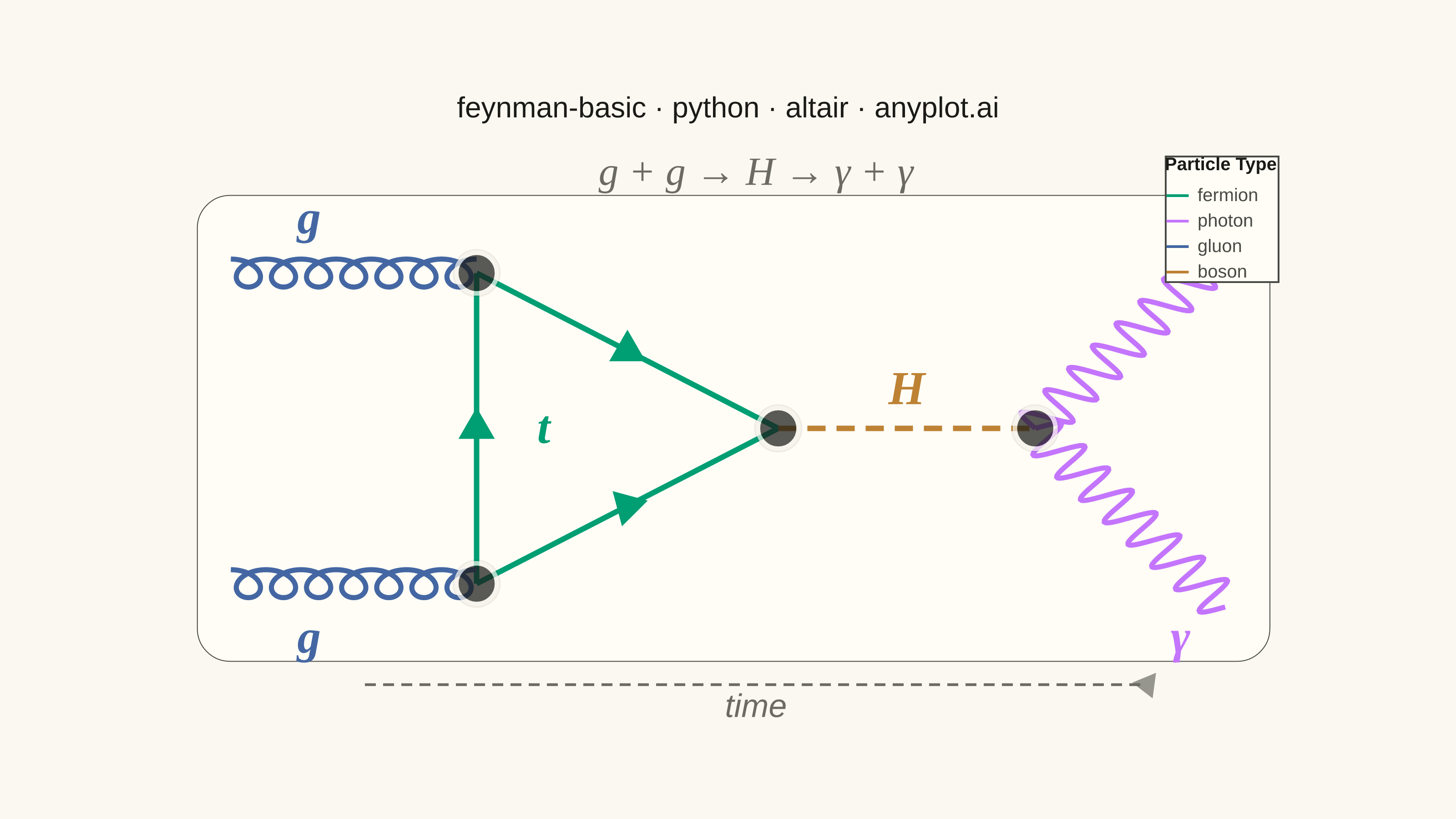
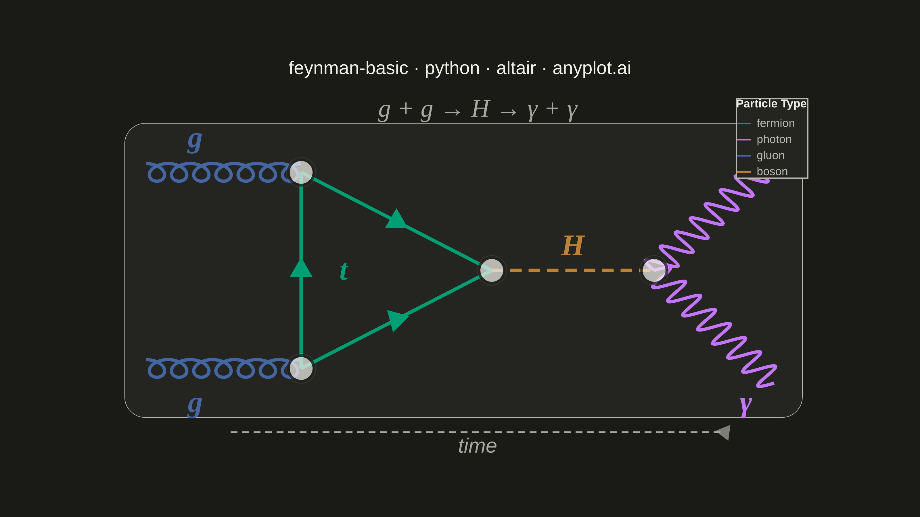
A Feynman diagram visualizes interactions between subatomic particles in quantum field theory. Different line styles represent different particle types: straight lines for fermions (electrons, quarks), wavy lines for photons, curly/looped lines for gluons, and dashed lines for scalar bosons (e.g., Higgs). Lines meet at vertices representing interaction points. Invented by Richard Feynman, these diagrams are both a computational tool and a cultural icon of modern physics.
""" anyplot.ai
feynman-basic: Feynman Diagram for Particle Interactions
Library: altair 6.1.0 | Python 3.13.13
Quality: 96/100 | Updated: 2026-06-03
"""

import os

import altair as alt
import numpy as np
import pandas as pd
from PIL import Image


# Theme tokens — Imprint palette chrome
THEME = os.getenv("ANYPLOT_THEME", "light")
PAGE_BG = "#FAF8F1" if THEME == "light" else "#1A1A17"
ELEVATED_BG = "#FFFDF6" if THEME == "light" else "#242420"
INK = "#1A1A17" if THEME == "light" else "#F0EFE8"
INK_SOFT = "#4A4A44" if THEME == "light" else "#B8B7B0"
INK_MUTED = "#6B6A63" if THEME == "light" else "#A8A79F"

# Imprint palette positions 1-4 mapped to the four particle types
color_scale = alt.Scale(
    domain=["fermion", "photon", "gluon", "boson"], range=["#009E73", "#C475FD", "#4467A3", "#BD8233"]
)

# Higgs boson production via gluon fusion: g + g → [t loop] → H → γ + γ
# All 4 particle types: fermion (straight+arrows), photon (wavy), gluon (curly), boson (dashed)

# Vertex positions spread across canvas
v1 = (2.5, 5.5)  # upper-left triangle vertex (g-t-t)
v2 = (2.5, 1.5)  # lower-left triangle vertex (g-t-t)
v3 = (5.2, 3.5)  # right triangle vertex (t-t-H)
v4 = (7.5, 3.5)  # Higgs decay vertex (H-γ-γ)

x_scale = alt.Scale(domain=[-0.3, 9.8])
y_scale = alt.Scale(domain=[-0.3, 7.2])

highlight = alt.selection_point(fields=["particle_type"], bind="legend")
opacity_cond = alt.condition(highlight, alt.value(1.0), alt.value(0.25))

# Straight lines: fermion triangle edges + dashed Higgs boson propagator
fermion_edges = [(v1, v2, "t1"), (v2, v3, "t2"), (v3, v1, "t3")]
straight_df = pd.DataFrame(
    [
        {"x": f[0], "y": f[1], "x2": t[0], "y2": t[1], "particle_type": "fermion", "label": "t", "line_id": pid}
        for f, t, pid in fermion_edges
    ]
    + [{"x": v3[0], "y": v3[1], "x2": v4[0], "y2": v4[1], "particle_type": "boson", "label": "H", "line_id": "H"}]
)

# Fermion direction arrows at edge midpoints
arrows_df = pd.DataFrame(
    [
        {
            "x": (f[0] + t[0]) / 2,
            "y": (f[1] + t[1]) / 2,
            "angle": np.degrees(np.arctan2(t[1] - f[1], t[0] - f[0])),
            "particle_type": "fermion",
            "label": "t",
        }
        for f, t, _ in fermion_edges
    ]
)

# Wavy paths (photon) — sinusoidal transverse offset
n_wavy = 200
wavy_paths = []
for x0, y0, x1, y1, lid in [(*v4, 9.2, 5.8, "γ1"), (*v4, 9.2, 1.2, "γ2")]:
    t = np.linspace(0, 1, n_wavy)
    dx, dy = x1 - x0, y1 - y0
    length = np.hypot(dx, dy)
    nx, ny = -dy / length, dx / length
    offset = 0.22 * np.sin(2 * np.pi * 8 * t)
    wavy_paths.append(
        pd.DataFrame(
            {
                "x": x0 + t * dx + offset * nx,
                "y": y0 + t * dy + offset * ny,
                "order": np.arange(n_wavy),
                "particle_type": "photon",
                "label": "γ",
                "line_id": lid,
            }
        )
    )

# Curly paths (gluon) — helical loop offset
n_curly, n_loops, loop_r = 400, 7, 0.18
curly_paths = []
for x0, y0, x1, y1, lid in [(0.3, 5.5, *v1, "g1"), (0.3, 1.5, *v2, "g2")]:
    dx, dy = x1 - x0, y1 - y0
    length = np.hypot(dx, dy)
    tx, ty = dx / length, dy / length
    nx, ny = -ty, tx
    theta = np.linspace(0, n_loops * 2 * np.pi, n_curly)
    base = np.linspace(0, length, n_curly)
    curly_paths.append(
        pd.DataFrame(
            {
                "x": x0 + (base + loop_r * np.sin(theta)) * tx + loop_r * np.cos(theta) * nx,
                "y": y0 + (base + loop_r * np.sin(theta)) * ty + loop_r * np.cos(theta) * ny,
                "order": np.arange(n_curly),
                "particle_type": "gluon",
                "label": "g",
                "line_id": lid,
            }
        )
    )

path_df = pd.concat(wavy_paths + curly_paths, ignore_index=True)

# Particle labels colored by type
label_df = pd.DataFrame(
    [
        {"x": 3.1, "y": 3.5, "label": "t", "particle_type": "fermion"},
        {"x": (v3[0] + v4[0]) / 2, "y": v3[1] + 0.5, "label": "H", "particle_type": "boson"},
        {"x": 1.0, "y": 6.2, "label": "g", "particle_type": "gluon"},
        {"x": 1.0, "y": 0.8, "label": "g", "particle_type": "gluon"},
        {"x": 8.8, "y": 6.2, "label": "γ", "particle_type": "photon"},
        {"x": 8.8, "y": 0.8, "label": "γ", "particle_type": "photon"},
    ]
)

# Vertex interaction points
vertex_df = pd.DataFrame(
    [
        {"x": v1[0], "y": v1[1], "vertex": "g-t-t"},
        {"x": v2[0], "y": v2[1], "vertex": "g-t-t"},
        {"x": v3[0], "y": v3[1], "vertex": "t-t-H"},
        {"x": v4[0], "y": v4[1], "vertex": "H-γ-γ"},
    ]
)

process_df = pd.DataFrame([{"x": 5.0, "y": 6.8, "text": "g + g  →  H  →  γ + γ"}])
time_line_df = pd.DataFrame([{"x": 1.5, "y": 0.2, "x2": 8.5, "y2": 0.2}])
time_arrow_df = pd.DataFrame([{"x": 8.5, "y": 0.2, "angle": 90}])
time_label_df = pd.DataFrame([{"x": 5.0, "y": -0.1, "label": "time"}])

# Subtle elevated background panel for the interaction region
bg_df = pd.DataFrame([{"x": 0.0, "y": 0.5, "x2": 9.6, "y2": 6.5}])
bg_layer = (
    alt.Chart(bg_df)
    .mark_rect(color=ELEVATED_BG, cornerRadius=18, stroke=INK_SOFT, strokeWidth=0.5)
    .encode(x=alt.X("x:Q", scale=x_scale, axis=None), y=alt.Y("y:Q", scale=y_scale, axis=None), x2="x2:Q", y2="y2:Q")
)

straight_layer = (
    alt.Chart(straight_df)
    .mark_rule(strokeWidth=3)
    .encode(
        x=alt.X("x:Q", scale=x_scale, axis=None),
        y=alt.Y("y:Q", scale=y_scale, axis=None),
        x2="x2:Q",
        y2="y2:Q",
        color=alt.Color(
            "particle_type:N",
            scale=color_scale,
            legend=alt.Legend(title="Particle Type", symbolSize=150, orient="top-right", offset=8),
        ),
        strokeDash=alt.StrokeDash(
            "particle_type:N", scale=alt.Scale(domain=["fermion", "boson"], range=[[1, 0], [10, 6]]), legend=None
        ),
        opacity=opacity_cond,
        tooltip=[alt.Tooltip("label:N", title="Particle"), alt.Tooltip("particle_type:N", title="Type")],
    )
    .add_params(highlight)
)

path_layer = (
    alt.Chart(path_df)
    .mark_line(strokeWidth=2.8)
    .encode(
        x=alt.X("x:Q", scale=x_scale, axis=None),
        y=alt.Y("y:Q", scale=y_scale, axis=None),
        color=alt.Color("particle_type:N", scale=color_scale, legend=None),
        detail="line_id:N",
        order="order:Q",
        opacity=opacity_cond,
        tooltip=[alt.Tooltip("label:N", title="Particle"), alt.Tooltip("particle_type:N", title="Type")],
    )
    .add_params(highlight)
)

arrow_layer = (
    alt.Chart(arrows_df)
    .mark_point(shape="triangle", size=400, filled=True)
    .encode(
        x=alt.X("x:Q", scale=x_scale, axis=None),
        y=alt.Y("y:Q", scale=y_scale, axis=None),
        angle=alt.Angle("angle:Q"),
        color=alt.Color("particle_type:N", scale=color_scale, legend=None),
        opacity=opacity_cond,
    )
    .add_params(highlight)
)

vertex_shadow = (
    alt.Chart(vertex_df)
    .mark_circle(size=700, color=INK, opacity=0.08)
    .encode(x=alt.X("x:Q", scale=x_scale, axis=None), y=alt.Y("y:Q", scale=y_scale, axis=None))
)

vertex_layer = (
    alt.Chart(vertex_df)
    .mark_circle(size=500, color=INK, stroke=PAGE_BG, strokeWidth=2.5)
    .encode(
        x=alt.X("x:Q", scale=x_scale, axis=None),
        y=alt.Y("y:Q", scale=y_scale, axis=None),
        tooltip=[alt.Tooltip("vertex:N", title="Interaction")],
    )
)

label_layer = (
    alt.Chart(label_df)
    .transform_calculate(description="datum.label + ' (' + datum.particle_type + ')'")
    .mark_text(fontSize=26, fontWeight="bold", font="serif", fontStyle="italic")
    .encode(
        x=alt.X("x:Q", scale=x_scale, axis=None),
        y=alt.Y("y:Q", scale=y_scale, axis=None),
        text="label:N",
        color=alt.Color("particle_type:N", scale=color_scale, legend=None),
        opacity=opacity_cond,
        tooltip=[alt.Tooltip("description:N", title="Particle")],
    )
    .add_params(highlight)
)

process_layer = (
    alt.Chart(process_df)
    .mark_text(fontSize=22, font="serif", fontStyle="italic", color=INK_MUTED)
    .encode(x=alt.X("x:Q", scale=x_scale, axis=None), y=alt.Y("y:Q", scale=y_scale, axis=None), text="text:N")
)

time_line_layer = (
    alt.Chart(time_line_df)
    .mark_rule(strokeWidth=1.5, color=INK_MUTED, strokeDash=[6, 4])
    .encode(x=alt.X("x:Q", scale=x_scale, axis=None), y=alt.Y("y:Q", scale=y_scale, axis=None), x2="x2:Q", y2="y2:Q")
)

time_arrow_layer = (
    alt.Chart(time_arrow_df)
    .mark_point(shape="triangle", size=200, filled=True, color=INK_MUTED)
    .encode(
        x=alt.X("x:Q", scale=x_scale, axis=None), y=alt.Y("y:Q", scale=y_scale, axis=None), angle=alt.Angle("angle:Q")
    )
)

time_label_layer = (
    alt.Chart(time_label_df)
    .mark_text(fontSize=18, color=INK_MUTED, fontStyle="italic")
    .encode(x=alt.X("x:Q", scale=x_scale, axis=None), y=alt.Y("y:Q", scale=y_scale, axis=None), text="label:N")
)

# Title: 44 chars — shorter than 67-char baseline, keep at default 16px
title_str = "feynman-basic · python · altair · anyplot.ai"

chart = (
    alt.layer(
        bg_layer,
        straight_layer,
        path_layer,
        arrow_layer,
        vertex_shadow,
        vertex_layer,
        label_layer,
        process_layer,
        time_line_layer,
        time_arrow_layer,
        time_label_layer,
    )
    .properties(
        width=620,
        height=320,
        background=PAGE_BG,
        title=alt.Title(title_str, fontSize=16, fontWeight="normal", anchor="middle", color=INK, offset=10),
    )
    .configure_view(fill=PAGE_BG, strokeWidth=0)
    .configure_axis(
        domainColor=INK_SOFT, tickColor=INK_SOFT, gridColor=INK, gridOpacity=0.15, labelColor=INK_SOFT, titleColor=INK
    )
    .configure_title(color=INK)
    .configure_legend(
        fillColor=ELEVATED_BG,
        strokeColor=INK_SOFT,
        labelColor=INK_SOFT,
        titleColor=INK,
        titleFontSize=10,
        labelFontSize=10,
    )
)

# Save PNG and pad to exact 3200×1800 canvas
TW, TH = 3200, 1800
chart.save(f"plot-{THEME}.png", scale_factor=4.0)
_img = Image.open(f"plot-{THEME}.png").convert("RGB")
_w, _h = _img.size
if _w > TW or _h > TH:
    raise SystemExit(
        f"altair vl-convert produced {_w}×{_h}, exceeds target {TW}×{TH}. "
        f"Shrink chart .properties(width=, height=) values and re-render."
    )
if _w < TW or _h < TH:
    _canvas = Image.new("RGB", (TW, TH), PAGE_BG)
    _canvas.paste(_img, ((TW - _w) // 2, (TH - _h) // 2))
    _canvas.save(f"plot-{THEME}.png")

chart.save(f"plot-{THEME}.html")
Runnable source as JSON, for any HTTP client: https://api.anyplot.ai/specs/feynman-basic/altair/code. Any spec id and library id listed in llms-full.txt fit the same URL shape; every URL below is complete and callable.
{
  "spec_id": "feynman-basic",
  "language": "python",
  "library": "altair",
  "page": "https://anyplot.ai/feynman-basic/python/altair",
  "hub": "https://anyplot.ai/feynman-basic",
  "code_json": "https://api.anyplot.ai/specs/feynman-basic/altair/code",
  "spec_json": "https://api.anyplot.ai/specs/feynman-basic",
  "render_light_png": "https://storage.googleapis.com/anyplot-images/plots/feynman-basic/python/altair/plot-light.png",
  "render_dark_png": "https://storage.googleapis.com/anyplot-images/plots/feynman-basic/python/altair/plot-dark.png",
  "interactive_light_html": "https://storage.googleapis.com/anyplot-images/plots/feynman-basic/python/altair/plot-light.html",
  "interactive_dark_html": "https://storage.googleapis.com/anyplot-images/plots/feynman-basic/python/altair/plot-dark.html",
  "quality_score": 96.0,
  "license": "MIT",
  "guide": "https://anyplot.ai/llms.txt"
}
Part of Feynman Diagram for Particle Interactions on anyplot.ai.